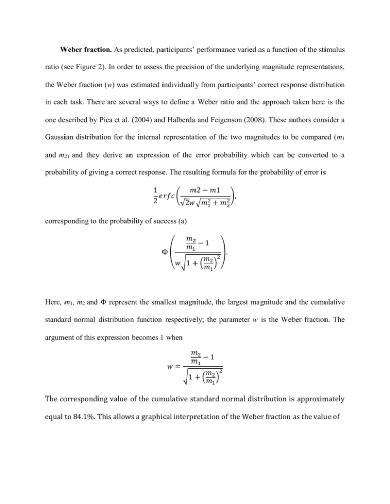
Weber fraction. As predicted, participants’ performance varied as a function of the stimulus
ratio (see Figure 2). In order to assess the precision of the underlying magnitude representations,
the Weber fraction (w) was estimated individually from participants’ correct response distribution
in each task. There are several ways to define a Weber ratio and the approach taken here is the
one described by Pica et al. (2004) and Halberda and Feigenson (2008). These authors consider a
Gaussian distribution for the internal representation of the two magnitudes to be compared (m1
and m2) and they derive an expression of the error probability which can be converted to a
probability of giving a correct response. The resulting formula for the probability of error is
1
𝑚2 − 𝑚1
𝑒𝑟𝑓𝑐 (
),
2
√2𝑤 √𝑚12 + 𝑚22
corresponding to the probability of success (a)
Φ
𝑚2
𝑚1 − 1
𝑚 2
𝑤√1 + ( 2 )
𝑚1 )
(
.
Here, m1, m2 and Φ represent the smallest magnitude, the largest magnitude and the cumulative
standard normal distribution function respectively; the parameter w is the Weber fraction. The
argument of this expression becomes 1 when
𝑤=
𝑚2
𝑚1 − 1
𝑚2 2
𝑚1 )
√1 + (
The corresponding value of the cumulative standard normal distribution is approximately
equal to 84.1%. This allows a graphical interpretation of the Weber fraction as the value of
𝑚2
𝑚1 − 1
𝜌=
𝑚2 2
𝑚1 )
√1 + (
at which the success rate is Φ(1) ≈ 84.14%. This can be used to determine the Weber
fraction empirically if the corresponding experiments included magnitude ratios 𝑚2 /𝑚1
whose corresponding success rates surround and are near to 84.14%. The method used
here for determining the Weber fraction is the method of the maximum likelihood. At any
value 𝜌𝑖 corresponding to a magnitude ratio, the probability of observing 𝑘_𝑖 successes on
𝑛𝑖 test items is given by a binomial distribution
𝑛𝑖
𝑛𝑖 −𝑘𝑖
(𝑘 ) 𝑝𝑖 (𝑤)𝑘𝑖 (1 − 𝑝𝑖 (𝑤))
𝑖
where 𝑝𝑖(𝑤) = Φ(𝜌𝑖 /𝑤). This yields the combined likelihood over all ratios
𝑛𝑖
𝑛𝑖 −𝑘𝑖
𝐿𝑖𝑘(𝑤; 𝑑𝑎𝑡𝑎) = ∏ (𝑘 ) 𝑝𝑖 (𝑤)𝑘𝑖 (1 − 𝑝𝑖 (𝑤))
.
𝑖
This likelihood can now be maximized (more conveniently on the log scale) to determine the
maximum likelihood estimate of w. It is clear that such an estimate is ill-defined when the rate of
correct responses for all magnitude ratios is much lower than 84.13%. In such cases the
maximum likelihood estimate of w may turn out unbounded or unreasonably high. This can be
avoided by adding a magnitude ratio at which all subjects obtain nearly perfect results. In our
study, this was implemented as a pre-test. Here the magnitude ratio was 3 and obtaining at least 5
out of 6 correct responses was the entry criterion for the main trial. The probability of obtaining
at least 5 out of 6 correct responses at a magnitude ratio of 3 is
6 ⋅ 𝑝𝑖 (𝑤)5 ⋅ (1 − 𝑝𝑖 (𝑤)) + 𝑝𝑖 (𝑤)6 = 𝑝𝑖 (𝑤)5 (6 − 5 ⋅ 𝑝𝑖 (𝑤)5 )
which can be added to the likelihood and serves to stabilize the calculation. This method permits
therefore to estimate individual Weber fractions for all individuals who passed the pre-test. Note
that the pre-test can add a bias to the estimation when the true Weber fraction is very large. Here
the probability to pass the pre-test is low and therefore subjects who have very low abilities to
discriminate are excluded. In order to assess this bias, we carried out a simulation study. This
simulation study showed no or almost no bias for Weber fractions between 0.05 and 0.5. For
Weber fractions above 0.6 (corresponding to a magnitude ratio of almost 3/1), bias increases and
becomes non-negligible above 0.7. This is that the procedure under-estimates the Weber fraction
for very severely impaired subjects. In the context of the present study, such subjects were not
part of the target population. The abovementioned estimation bias is therefore not relevant in our
situation.