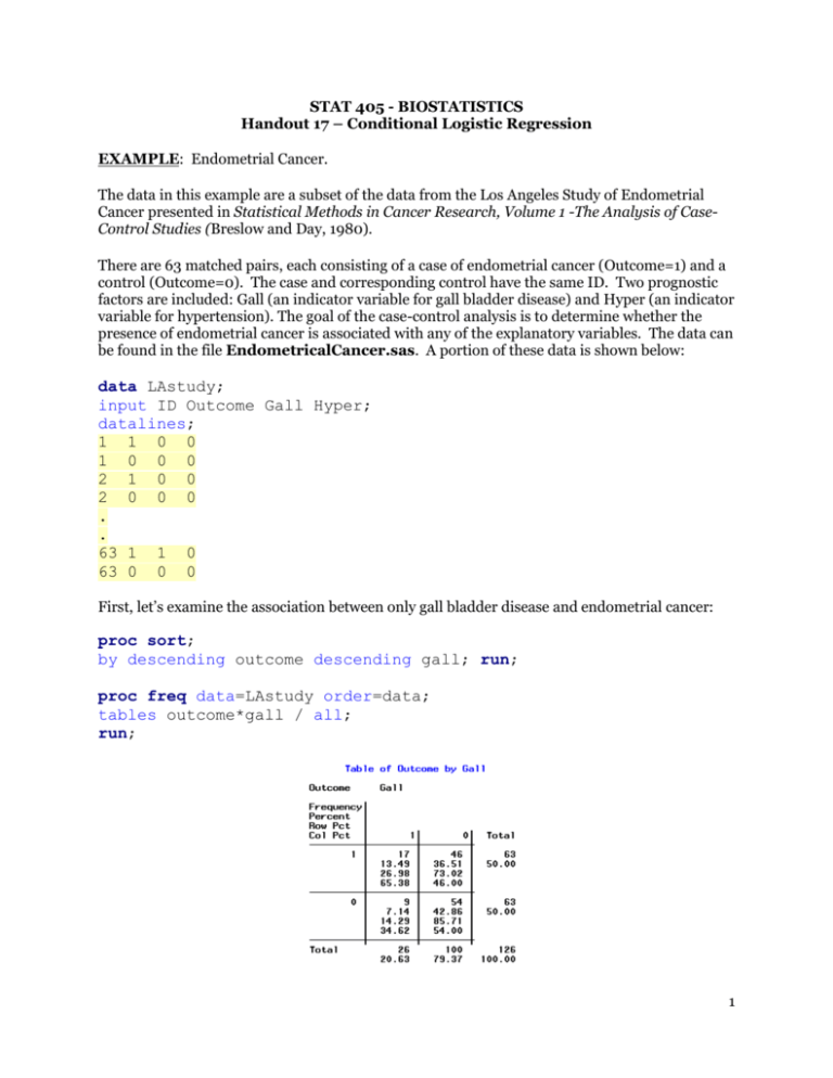
STAT 405 - BIOSTATISTICS
Handout 17 – Conditional Logistic Regression
EXAMPLE: Endometrial Cancer.
The data in this example are a subset of the data from the Los Angeles Study of Endometrial
Cancer presented in Statistical Methods in Cancer Research, Volume 1 -The Analysis of CaseControl Studies (Breslow and Day, 1980).
There are 63 matched pairs, each consisting of a case of endometrial cancer (Outcome=1) and a
control (Outcome=0). The case and corresponding control have the same ID. Two prognostic
factors are included: Gall (an indicator variable for gall bladder disease) and Hyper (an indicator
variable for hypertension). The goal of the case-control analysis is to determine whether the
presence of endometrial cancer is associated with any of the explanatory variables. The data can
be found in the file EndometricalCancer.sas. A portion of these data is shown below:
data LAstudy;
input ID Outcome Gall Hyper;
datalines;
1 1 0 0
1 0 0 0
2 1 0 0
2 0 0 0
.
.
63 1 1 0
63 0 0 0
First, let’s examine the association between only gall bladder disease and endometrial cancer:
proc sort;
by descending outcome descending gall; run;
proc freq data=LAstudy order=data;
tables outcome*gall / all;
run;
1
Note that we obtain the same odds ratio using logistic regression:
proc logistic data=LAstudy;
class Gall(param=ref ref='0');
model outcome(event='1') = Gall/ clodds=wald;
run;
Questions:
1. Interpret the point estimate of the odds ratio in the context of the problem.
2. Is gall bladder disease a significant predictor for the presence of endometrial cancer?
Explain.
3. Does this analysis account for the matched pairs in any way? Explain.
2
Another Approach: Reviewing McNemar’s Test
To account for the matched pairs, we could consider using McNemar’s test. To do this, we will
classify pairs according to whether or not the members of that pair had gall bladder disease. We
organize the data differently to set up this contingency table:
data LAstudy2;
input ID Case_gall Case_hyper Control_gall Control_hyper outcome;
datalines;
1
0
0
0
0
0
2
0
0
0
0
0
.
.
63
1
0
0
0
0
proc freq data=LAstudy2;
tables case_gall*control_gall;
exact mcnem;
run;
Estimation of Odds Ratio in Matched-Pair Studies:
It can be shown that for matched-pair data,

OR  n A
nB
where nA = number of discordant pairs of type A and nB = number of discordant pairs of type B.
3
Questions:
1. Find the odds ratio for endometrial cancer associated with the presence of gall bladder
disease (using the analysis that accounts for matching).
2. How does this compare to the odds ratio computed in the analysis not accounting for
matched pairs?
3. Can you use McNemar’s test to compute an odds ratio associated with the presence of
gall bladder disease after adjusting for hypertension? If not, how would you do this?
Conditional Logistic Regression
Note that we could fit the following model in PROC LOGISTIC as an attempt to account for the
matched pairs:
proc logistic data=LAstudy descending;
class id Gall;
model outcome = id Gall;
run;
This approach is NOT RECOMMENDED for the following reasons:

How many parameters would be added to the model by including an id effect? Recall
that there are 63 subjects!

When the number of parameters in the model is large relative to the sample size, the
maximum likelihood estimates are BIASED, which leads to biased estimates of the odds
ratios.
A better approach is to use conditional logistic regression. It turns out that the conditional
likelihood for the matched pairs data is the unconditional likelihood for a logistic regression
model where the response is always equal to some constant value, the covariate values are equal
to the differences between the value for the case and the control, and there is no intercept.
4
So, we can use PROC LOGISTIC for conditional logistic regression if we take the following steps:
1. Create one observation per matched pair and make the predictor variables the
differences between the case values and the control values.
2. Set the response variable equal to any constant value.
3. Set the model intercept equal to zero.
This is carried out is PROC LOGISTIC as follows:
data LAstudy2;
input ID Case_gall Case_hyper Control_gall Control_hyper outcome;
Gall = Case_gall - Control_gall;
Hyper = Case_hyper - Control_hyper;
datalines;
1
0
0
0
0
0
2
0
0
0
0
0
.
63
1
0
0
0
0
;
proc logistic data=LAstudy2;
model outcome = Gall / noint clodds=wald;
run;
5
Questions:
1. How does this odds ratio compare to the odds ratio computed on page 4?
2.
Is gall bladder disease a significant predictor for endometrial cancer? Explain.
Finally, we can fit a conditional logistic regression model which includes both gall bladder and
hypertension as predictors:
data LAstudy2;
input ID Case_gall Case_hyper Control_gall Control_hyper outcome;
Gall = Case_gall - Control_gall;
Hyper = Case_hyper - Control_hyper;
datalines;
1
0
0
0
0
0
2
0
0
0
0
0
.
63
1
0
0
0
0
;
proc logistic data=LAstudy2;
model outcome = Gall Hyper / noint clodds=wald;
run;
6
Another Approach with PROC LOGISTIC
Note that it is not necessary that you rearrange the data so that there is one observation per
matched pair. You can also fit the conditional logistic regression model as follows:
data LAstudy;
input ID Outcome Gall Hyper;
datalines;
1 1 0 0
1 0 0 0
2 1 0 0
2 0 0 0
.
.
63 1 1 0
63 0 0 0
;
proc logistic data=LAstudy descending;
class Gall(param=ref ref='0') Hyper(param=ref ref='0');
strata id;
model outcome(event='1') = Gall Hyper / clodds=wald noint;
run;
Questions:
1. What do you conclude from this analysis?
2. How much did the odds ratio associated with gall bladder disease change after adjusting
for hypertension? Is this what you expected? Explain.
7