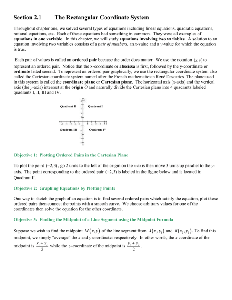
Section 2.1
The Rectangular Coordinate System
Throughout chapter one, we solved several types of equations including linear equations, quadratic equations,
rational equations, etc. Each of these equations had something in common. They were all examples of
equations in one variable. In this chapter, we will study equations involving two variables. A solution to an
equation involving two variables consists of a pair of numbers, an x-value and a y-value for which the equation
is true.
Each pair of values is called an ordered pair because the order does matter. We use the notation  x, y  to
represent an ordered pair. Notice that the x-coordinate or abscissa is first, followed by the y-coordinate or
ordinate listed second. To represent an ordered pair graphically, we use the rectangular coordinate system also
called the Cartesian coordinate system named after the French mathematician René Descartes. The plane used
in this system is called the coordinate plane or Cartesian plane. The horizontal axis (x-axis) and the vertical
axis (the y-axis) intersect at the origin O and naturally divide the Cartesian plane into 4 quadrants labeled
quadrants I, II, III and IV.
Quadrant II
Quadrant III
Quadrant I
Quadrant IV
Objective 1: Plotting Ordered Pairs in the Cartesian Plane
To plot the point (2,3) , go 2 units to the left of the origin on the x-axis then move 3 units up parallel to the yaxis. The point corresponding to the ordered pair (2,3) is labeled in the figure below and is located in
Quadrant II.
Objective 2: Graphing Equations by Plotting Points
One way to sketch the graph of an equation is to find several ordered pairs which satisfy the equation, plot those
ordered pairs then connect the points with a smooth curve. We choose arbitrary values for one of the
coordinates then solve the equation for the other coordinate.
Objective 3: Finding the Midpoint of a Line Segment using the Midpoint Formula
Suppose we wish to find the midpoint M  x, y  of the line segment from A  x1 , y1  and B  x2 , y2  . To find this
midpoint, we simply “average” the x and y coordinates respectively. In other words, the x coordinate of the
x x
y  y2
midpoint is 1 2 while the y-coordinate of the midpoint is 1
.
2
2
B  x2 , y2 
M  x, y 
A  x1 , y1 
Midpoint Formula
The midpoint of the line segment from A  x1 , y1  to B  x2 , y2  is
 x1  x2 y1  y2 
,

.
2 
 2
Objective 4: Finding the Distance between Two Points using the Distance Formula
Recall that the Pythagorean Theorem states that the sum of the squares of the two sides of a right triangle is
equal to the square of the hypotenuse or a 2  b 2  c 2 .
c
b
The Pythagorean
Theorem a2  b2  c2
a
We can use the Pythagorean Theorem to find the distance between any two points in a plane. To find the length
d  A, B  of the line segment AB, consider the point C  x1 , y2  which is on the same vertical line segment as
point A and the same horizontal line segment as point B. The triangle formed by points A, B and C is a right
triangle whose hypotenuse has length d  A, B  . The horizontal leg of the triangle has length a  x2  x1 while
the vertical leg of the triangle has length b  y2  y1 .
x2  x1  y2  y1   d ( A, B )  .
2
2
2
a2
b2
 d ( A, B)
2
c2
 x2  x1  y2  y1
2
2
d ( A, B)   x2  x1  y2  y1
2
A  x1 , y1 
Use the Pythagorean Theorem.
2
d ( A, B)
b  y2  y1
Use the Square Root Property.
But since distance cannot be negative, exclude  x2  x1  y2  y1 .
2
d ( A, B) 
x2  x1  y2  y1
d ( A, B) 
 x2  x1    y2  y1 
2
2
2
2
B  x2 , y2 
Use the positive square root only.
2
For any quantity A, A  A2 .
2
The Distance Formula
The distance between any two points A  x1 , y1  and B  x2 , y2  is given by the formula
d ( A, B) 
 x2  x1    y2  y1 
2
2
a  x2  x1
C  x1 , y2 