Name:_______________________________________
Exam#2
Applied Numerical Weather Prediction
Due: noon, 5 May 2015
NOTE: All work is to be completed individually, without consulting any other person.
Project#21
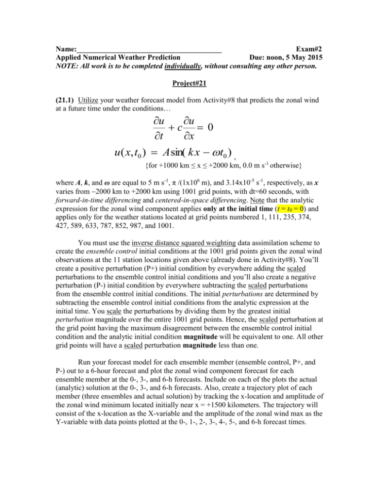
(21.1) Utilize your weather forecast model from Activity#8 that predicts the zonal wind
at a future time under the conditions…
u
u
c  0
t
x
u( x, t0 )  A sin( k x  t0 ) ,
{for +1000 km ≤ x ≤ +2000 km, 0.0 m s-1 otherwise}
where A, k, and ω are equal to 5 m s-1, π /(1x106 m), and 3.14x10-5 s-1, respectively, as x
varies from 2000 km to +2000 km using 1001 grid points, with dt=60 seconds, with
forward-in-time differencing and centered-in-space differencing. Note that the analytic
expression for the zonal wind component applies only at the initial time (t = t0 = 0) and
applies only for the weather stations located at grid points numbered 1, 111, 235, 374,
427, 589, 633, 787, 852, 987, and 1001.
You must use the inverse distance squared weighting data assimilation scheme to
create the ensemble control initial conditions at the 1001 grid points given the zonal wind
observations at the 11 station locations given above (already done in Activity#8). You’ll
create a positive perturbation (P+) initial condition by everywhere adding the scaled
perturbations to the ensemble control initial conditions and you’ll also create a negative
perturbation (P-) initial condition by everywhere subtracting the scaled perturbations
from the ensemble control initial conditions. The initial perturbations are determined by
subtracting the ensemble control initial conditions from the analytic expression at the
initial time. You scale the perturbations by dividing them by the greatest initial
perturbation magnitude over the entire 1001 grid points. Hence, the scaled perturbation at
the grid point having the maximum disagreement between the ensemble control initial
condition and the analytic initial condition magnitude will be equivalent to one. All other
grid points will have a scaled perturbation magnitude less than one.
Run your forecast model for each ensemble member (ensemble control, P+, and
P-) out to a 6-hour forecast and plot the zonal wind component forecast for each
ensemble member at the 0-, 3-, and 6-h forecasts. Include on each of the plots the actual
(analytic) solution at the 0-, 3-, and 6-h forecasts. Also, create a trajectory plot of each
member (three ensembles and actual solution) by tracking the x-location and amplitude of
the zonal wind minimum located initially near x = +1500 kilometers. The trajectory will
consist of the x-location as the X-variable and the amplitude of the zonal wind max as the
Y-variable with data points plotted at the 0-, 1-, 2-, 3-, 4-, 5-, and 6-h forecast times.
Name:_______________________________________
Exam#2
Applied Numerical Weather Prediction
Due: noon, 5 May 2015
NOTE: All work is to be completed individually, without consulting any other person.
Project#21 (continued)
[q21.2.1] Based on the results of your trajectory plot, would you conclude
that the ensemble system was “good” or “bad” at predicting the evolution of the
zonal wind maximum that starts near x = +1500 kilometers. Give reasons
supporting your conclusion.
[q21.2.2] What feature of the sinusoidal zonal wind field is not handled
well by the control forecast and isn’t accounted for in the simple perturbation
ensemble methodology such that the results of our ensemble system might be
less-than-desirable? Give reasons supporting your conclusion.