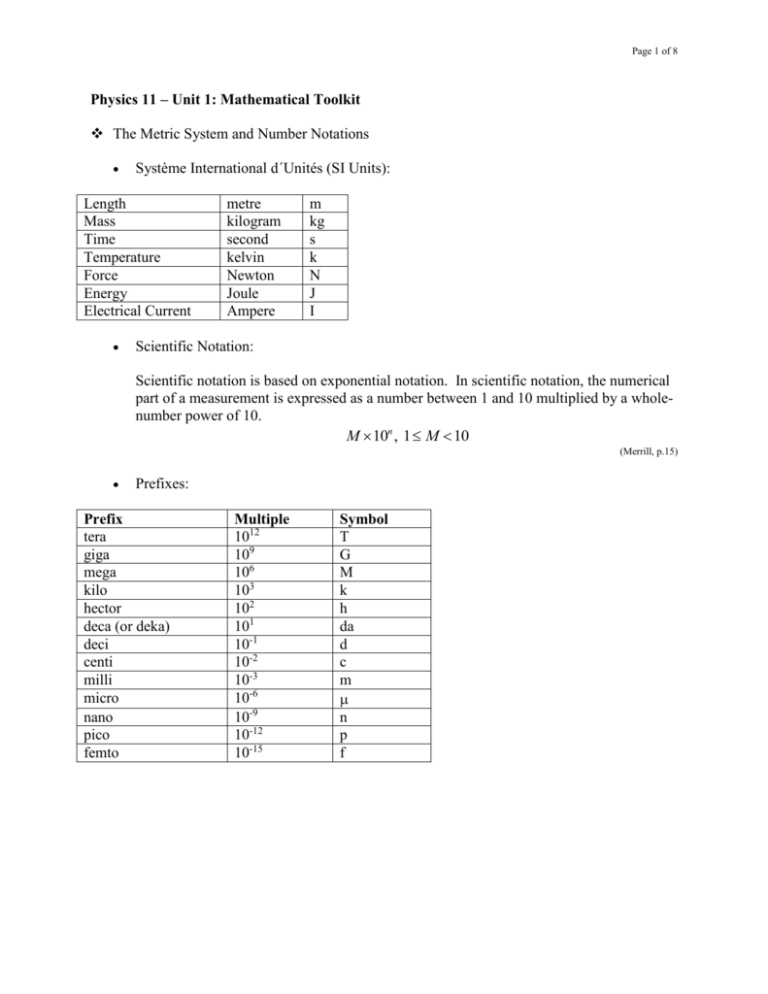
Page 1 of 8
Physics 11 – Unit 1: Mathematical Toolkit
 The Metric System and Number Notations

Système International d´Unités (SI Units):
Length
Mass
Time
Temperature
Force
Energy
Electrical Current

metre
kilogram
second
kelvin
Newton
Joule
Ampere
m
kg
s
k
N
J
I
Scientific Notation:
Scientific notation is based on exponential notation. In scientific notation, the numerical
part of a measurement is expressed as a number between 1 and 10 multiplied by a wholenumber power of 10.
M  10n , 1  M  10
(Merrill, p.15)

Prefixes:
Prefix
tera
giga
mega
kilo
hector
deca (or deka)
deci
centi
milli
micro
nano
pico
femto
Multiple
1012
109
106
103
102
101
10-1
10-2
10-3
10-6
10-9
10-12
10-15
Symbol
T
G
M
k
h
da
d
c
m

n
p
f
Page 2 of 8
 Uncertainty in Measurements

Precision and Accuracy:
-
Precision is the degree of exactness to which the measurement of a quantity can be
reproduced. The precision of an instrument is limited by the smallest division on the
measurement scale.
-
Accuracy is the extent to which a measured value agrees with the standard value of a
quantity. The accuracy of a measurement describes how well the result agrees with
an accepted value.
(Merrill, p. 21-22)
(a) precise and accurate

(b) precise but not accurate
(c) neither precise nor accurate
Significant Digits:
Significant digits are all the digits that are certain plus a digit that estimates the fraction
of the smallest division of the measuring scale. Follow these rules to decide if a digit is
significant:
1.
2.
3.
4.
Nonzero digits are always significant. e.g. 1234 – 4 s.d.
All final zeros after the decimal point are significant. e.g. 6.00 – 3 s.d.
Zeros between two other significant digits are always significant. e.g. 2005 – 4 s.d.
Zeros to the right of a whole number are considered to be ambiguous. e.g. 300 – 1 s.d.
(Merrill, p. 22-23)

Operations Using Significant Digits:
-
e.g.
The sum or difference of two values is as precise as the least precise value.
12.345
 1.23
13.575
 13.58
Page 3 of 8
-
e.g.
The number of significant digits in a product or quotient is the number in the factor
with the lesser number of significant digits.
12.345
 12345
.
15.2399025
 15.240
(Merrill, p. 24-25)

The Errors:
-
Random Error results when an estimate is made to obtain the last significant digit for
any measurement.
e.g. When measuring length, it is necessary to estimate between the marks on the
measuring tape. If thee marks are 1 cm apart, the random error will be greater and
the precision will be less than if the marks are 1 mm apart.
-
Systematic Error is associated with an inherent problem with the measuring system,
such as the presence of an interfering substance, incorrect calibration, or room
conditions.
e.g. If the balance is not zeroed at the beginning, all measurements will have a
systematic error; using a slightly worn metre stick will also introduce error.
-
% error
% error =
experimental value - accepted value
 100%
accepted value
e.g. When we measured the speed of sound, we found it to be 342 m/s. The accepted
values at the same temperature is 352 m/s.
342 - 352
 100% = - 2.84%
352
The negative sign indicates that our measured value was less than the accepted
value.
% error =
-
% difference
% difference =
difference in measurements
 100%
average measurement
e.g. If two measurements of the speed of sound are 342 m/s and 348 m/s. Their %
difference is:
6.00
% difference =
 100% = 2.00%
345
(Hirsch, Martindale, Bibla & Stewart, p. 565; Heath, Macnaughton & Martindale, p. 553-554)
Page 4 of 8
 Graphing Scientific Data

The procedures:
1. Choosing the Axes:
Determine which of the physical quantities is the dependent variable and which is the
independent variable. The independent variable is plotted on the horizontal axis and
the dependent variable on the vertical axis. (y versus x)
2. Scaling the Axes:
When choosing scales, spread the measured values across the graph paper as widely
as possible. The scales chosen must be easy to read and must have equal divisions.
Each axis is labeled with the symbol for what is being plotted and the unit.
3. Plotting the Date:
Find each data point and mark it with a small dot in pencil. Around each dot draw a
small circle not exceeding two small scale divisions in diameter. With a wellsharpened pencil, lightly draw in the smooth curve that best joins the small circles.
Do not try to force your line to go through all dots, since experimental error will
cause some points to be slightly off the smooth curve. If the points seem to lie on a
straight line, use a ruler, preferably a transparent one, so that you can see all the
points while selecting the best line. Sometimes a point obviously has no experimental
error, so the line must go through it.
(Heath, Macnaughton & Martindale, p. 554-555)

Linear Equations:
m
yR  y L
, y = mx + y0
xR  x L
m is the slope of line and y0 is the initial value on the vertical axis (y intercept)

Quadratic Equations:
y  cx 2  y0
c is vertical factor and y0 is the max. or mim. Value

Reciprocal Relations:
y
c
c
or y  2 , x  0
x
x
c is vertical factor

Radical Relations:
y  x, x  0
Page 5 of 8
 Proportioning Techniques
The statement of how one quantity varies in relation to another is called a proportionality
expression.
e.g.
Time (s)
Distance (m)
1
28
2
56
3
84
4
112
5
140
6
168
7
196
dt
e.g. The force of air resistance (F) on a moving body is related to the speed of the body (v) by
the proportion F  v2. If the speed triples, how many times greater is the force?
e.g. The cylindrical water tank holds 1.0  105 L of water. How much would it hold if all of
its dimensions were doubled?
 Manipulating Equations
Page 6 of 8
e.g. Find l, if T 
l
.
g
e.g. Find  i, if ni sin  i  nr sin  r .
e.g. Find d i, if
1
1 1
.


f d o di
e.g. Find v i, if v 2f  vi2  2ad .
 Conversion of Units
e.g. Changes 4.5 km to cm.
e.g. How many s are contained in 2.5 h?
e.g. Convert 80.0 km/s to m/s.
Physics 11 - Unit 1: Mathematic Toolkits: Practice
Page 7 of 8
Page 8 of 8