Additional File 1: Text S1
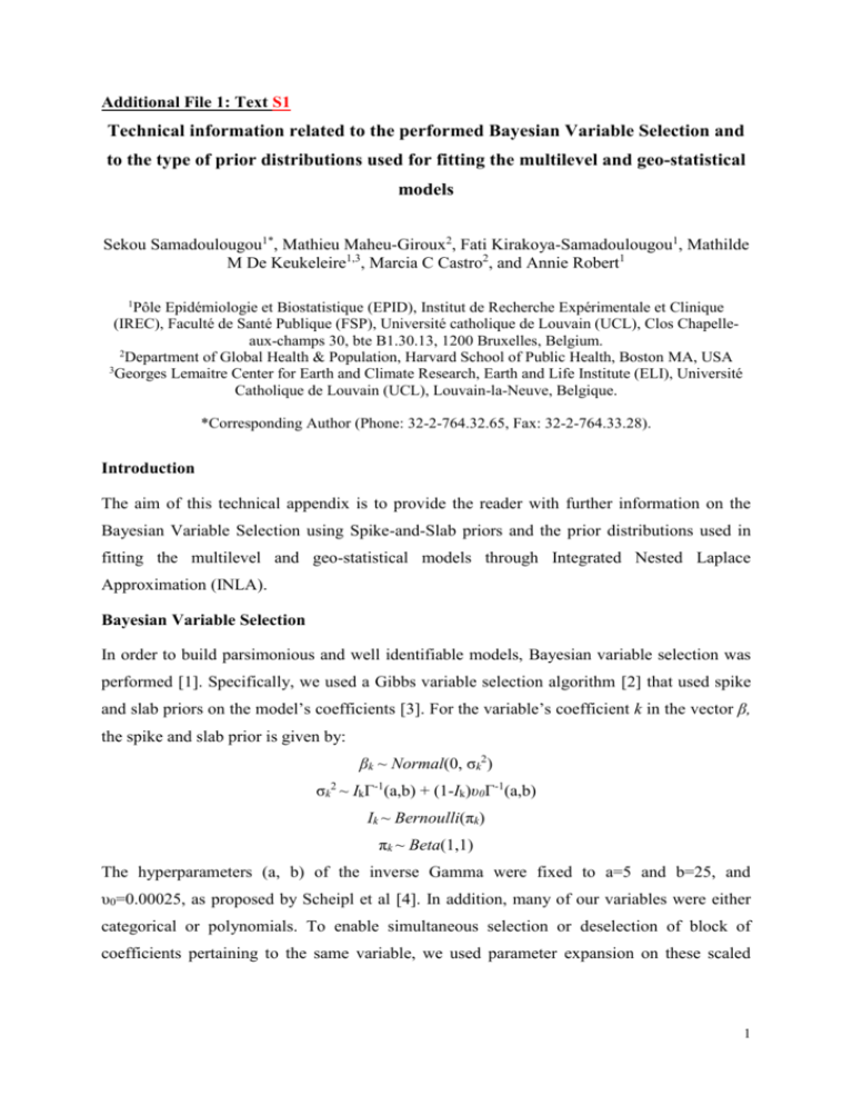
Technical information related to the performed Bayesian Variable Selection and
to the type of prior distributions used for fitting the multilevel and geo-statistical
models
Sekou Samadoulougou1*, Mathieu Maheu-Giroux2, Fati Kirakoya-Samadoulougou1, Mathilde
M De Keukeleire1,3, Marcia C Castro2, and Annie Robert1
1
Pôle Epidémiologie et Biostatistique (EPID), Institut de Recherche Expérimentale et Clinique
(IREC), Faculté de Santé Publique (FSP), Université catholique de Louvain (UCL), Clos Chapelleaux-champs 30, bte B1.30.13, 1200 Bruxelles, Belgium.
2
Department of Global Health & Population, Harvard School of Public Health, Boston MA, USA
3
Georges Lemaitre Center for Earth and Climate Research, Earth and Life Institute (ELI), Université
Catholique de Louvain (UCL), Louvain-la-Neuve, Belgique.
*Corresponding Author (Phone: 32-2-764.32.65, Fax: 32-2-764.33.28).
Introduction
The aim of this technical appendix is to provide the reader with further information on the
Bayesian Variable Selection using Spike-and-Slab priors and the prior distributions used in
fitting the multilevel and geo-statistical models through Integrated Nested Laplace
Approximation (INLA).
Bayesian Variable Selection
In order to build parsimonious and well identifiable models, Bayesian variable selection was
performed [1]. Specifically, we used a Gibbs variable selection algorithm [2] that used spike
and slab priors on the model’s coefficients [3]. For the variable’s coefficient k in the vector β,
the spike and slab prior is given by:
βk ~ Normal(0, σk2)
σk2 ~ IkΓ-1(a,b) + (1-Ik)υ0Γ-1(a,b)
Ik ~ Bernoulli(πk)
πk ~ Beta(1,1)
The hyperparameters (a, b) of the inverse Gamma were fixed to a=5 and b=25, and
υ0=0.00025, as proposed by Scheipl et al [4]. In addition, many of our variables were either
categorical or polynomials. To enable simultaneous selection or deselection of block of
coefficients pertaining to the same variable, we used parameter expansion on these scaled
1
normal mixture of inverse Gamma [4] to avoid oversampling block of coefficients around
zero [5]. This prior takes the following form for category h of variable βk:
βkh = ϕkξkh
ξkh ~ Normal(mkh, 1)
mkh = γhk – (1- γkh)
γkh ~ Bernoulli(0.5)
where ϕk is given a spike and slab prior, as described above. The best set of predictors was
identified using a model with independent random effect at the community level. Model
selection was performed using Markov Chain Monte Carlo (MCMC) simulations
implemented in JAGS [6]. An adaptive phase of 5,000 iterations and 5 chains of 35,000
iterations were used after discarding 5,000 iterations per chain as burn-in (inference was thus
based on 150,000 iterations). The ‘rjags’ and ‘CODA’ libraries were used to run JAGS within
the R statistical software [7] .
Prior distributions of the multilevel and geo-statistical models
The Bayesian model formulations described in the manuscript was completed using noninformative priors on all model hyperparameters and parameters. Specifically, all regression
parameters were assumed to have Gaussian distributions with mean of zero and precision of
0.001. Priors for the hyperparameters of the random effect at the community level were
defined on the logarithmic scale. That is, we assumed that the precision of the random effect
followed a logGamma(shape=1, scale=1e-5) distribution. For the spatially-structured random
effect of the geo-statistical model, the hyperparameters are the precision and spatial scale
parameter (κ) of the Matérn model. Again, both hyperparameters are defined on the
logarithmic scale and are given vague log-Normal prior distributions, where the prior medians
for the hyperparameter are chosen heuristically to match the domain’s spatial scale (see
Lindgren 2012 for more information – [8])
2
Additional References
1. Spiegelhalter DJ, Best NG, Carlin BP, Linde AVD: Bayesian measures of model complexity
and fit. Journal of the Royal Statistical Society: Series B( Statistical Methodology) 2002, 64:
583.
2. Dellaportas P FJaNI: On Bayesian Model andVariable Selection Using MCMC. Statistics
and Computing 2014, 12: 27-36.
3. Ishwaran H, Rao JS: Spike and slab variable selection: Frequentist and Bayesian strategies.
Ann Statist 2005, 33: 730-773.
4. Scheipl F, Fahrmeira L, Kneib T: Posterior consistency of Bayesian quantile regression
based on the misspecified asymmetric Laplace density. Journal of the American Statistical
Association 2012, 107: 1518-1532.
5. Gelman A vDAHZBJ: Using redundant parameters to fit hierarchical models. J Comput
Graph Statist 2008, 17: 95-122.
6. Plummer M: JAGS: A Program for Analysis of Bayesian Graphical Models Using Gibbs
Sampling. 2013:1-10.
7. Plummer M. rjags: Bayesian graphical models using MCMC. R package version 3-12.
http://CRAN.R-project.org/package=rjags . 2014.
8. Lindgren F. Continuous domain spatial models in R-INLA. The ISBA bulletin.
http://bayesian.org/bulletin , 14-20. 2012.
3