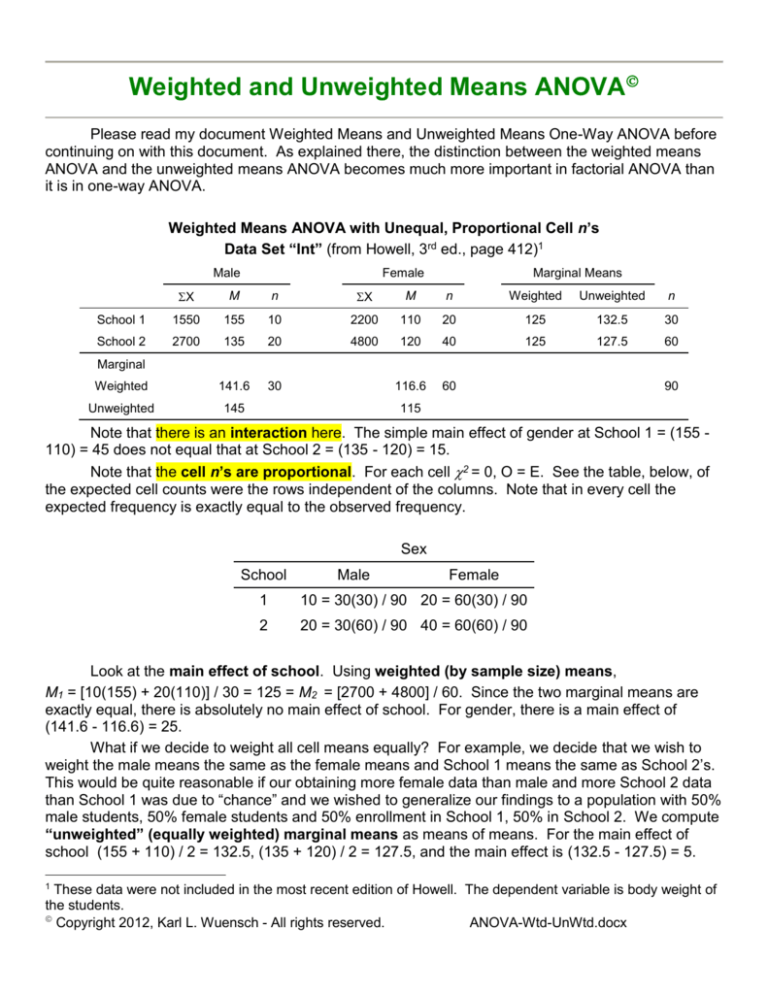
Weighted and Unweighted Means ANOVA
Please read my document Weighted Means and Unweighted Means One-Way ANOVA before
continuing on with this document. As explained there, the distinction between the weighted means
ANOVA and the unweighted means ANOVA becomes much more important in factorial ANOVA than
it is in one-way ANOVA.
Weighted Means ANOVA with Unequal, Proportional Cell n’s
Data Set “Int” (from Howell, 3rd ed., page 412)1
Male
Female
Marginal Means
X
M
n
X
M
n
Weighted
Unweighted
n
School 1
1550
155
10
2200
110
20
125
132.5
30
School 2
2700
135
20
4800
120
40
125
127.5
60
Weighted
141.6
30
116.6
60
Unweighted
145
Marginal
90
115
Note that there is an interaction here. The simple main effect of gender at School 1 = (155 110) = 45 does not equal that at School 2 = (135 - 120) = 15.
Note that the cell n’s are proportional. For each cell 2 = 0, O = E. See the table, below, of
the expected cell counts were the rows independent of the columns. Note that in every cell the
expected frequency is exactly equal to the observed frequency.
Sex
School
Male
Female
1
10 = 30(30) / 90 20 = 60(30) / 90
2
20 = 30(60) / 90 40 = 60(60) / 90
Look at the main effect of school. Using weighted (by sample size) means,
M1 = [10(155) + 20(110)] / 30 = 125 = M2 = [2700 + 4800] / 60. Since the two marginal means are
exactly equal, there is absolutely no main effect of school. For gender, there is a main effect of
(141.6 - 116.6) = 25.
What if we decide to weight all cell means equally? For example, we decide that we wish to
weight the male means the same as the female means and School 1 means the same as School 2’s.
This would be quite reasonable if our obtaining more female data than male and more School 2 data
than School 1 was due to “chance” and we wished to generalize our findings to a population with 50%
male students, 50% female students and 50% enrollment in School 1, 50% in School 2. We compute
“unweighted” (equally weighted) marginal means as means of means. For the main effect of
school (155 + 110) / 2 = 132.5, (135 + 120) / 2 = 127.5, and the main effect is (132.5 - 127.5) = 5.
1
These data were not included in the most recent edition of Howell. The dependent variable is body weight of
the students.

Copyright 2012, Karl L. Wuensch - All rights reserved.
ANOVA-Wtd-UnWtd.docx
2
This is not what we found with a weighted means approach, which indicated absolutely no effect of
school. Note that the size of the main effect of gender also varies with method of weighting the
means.
What if there were no interaction? For example,
Data Set 
Male
Female
Marginal Means
X
M
n
X
M
n
Weighted
Unweighted
n
School 1
1550
155
10
2800
140
20
145
147.5
30
School 2
2700
135
20
4800
120
40
125
127.5
60
Weighted
141.6
30
126.6
60
Unweighted
145
Marginal
90
130
(155 - 140) = (135 - 120)  no interaction. The main effect for school is (145 - 125) = 20 with
weighted means, = (147.5 - 127.5) = 20 for unweighted means. Choice of weighting method also has
no effect on the main effect of gender.
We have seen that even with proportional cell n’s the row and column effects are not
independent of any interaction effects present. If an interaction is present with such data, choice of
weighting techniques affects the results.
Computation of Weighted Means ANOVA Using Data Set “Int”
SSTOT = 81000 (given)
CM 
Y 2

N
SScells  
Tij2
nij
1550  2200  2700  48002
10  20  20  40
 CM 
 1406250
1550 2 2200 2 2700 2 4800 2



 CM 
10
20
20
40
1422750  1406250  16500
Ti 2
1550  2200  2700  4800  CM  0
 CM 
10  20
20  40
ni
2
SSSchool  
SSGender  
T j2
nj
2
2
2


1550  2700
2200  4800
 CM 

 CM  12500
10  20
20  40
SSerror  SSTOT  SScells  81000  16500  64500
SSSchool _ x _ Gender  SScells  SSSchool  SSGender  16500  0  12500  4000
3
Source
SS
df
MS
School
0
1
0
Gender
12500
1
12500
4000
1
4000
Error
64500
86
750
Total
81000
89
Interaction
F
0.0
p
1.000
16.6 < .001
5.3
.024
Interaction Analysis:
1550 2 2200 2 1550  2200 


 13500
10
20
10  20
F(1, 86) = 13500 / 750 = 18, p < .001.
2
SSGender _ at _ School _ 1 
2700 2 4800 2 2700  4800 
SSGender _ at _ School _ 2 


 3000
20
40
20  40
F(1, 86) = 3000 / 750 = 4, p = .049.
Significant gender effects at both schools, but a greater difference between male students and
female students at School 1 than at School 2.
------------------------------------ OR ------------------------------------2
1550 2 2700 2 1550  2700


 2666.6
10
20
10  20
F(1, 86) = 2666.6 / 750 = 3.5, p = .06.
2
SSSchool _ Male _ students 
2200 2 4800 2 2200  4800


 1333.3
20
40
20  40
F(1, 86) = 1333.3 / 750 = 1.7, p = .19.
Nonsignificant school differences for each gender, but trends in opposite directions [Sch 1 >
Sch 2 for male students, Sch 1 < Sch 2 for female students].
2
SSSchool _ Female _ students 
Traditional Unweighted Means ANOVA
One simple way to weight the cell means equally involves using the harmonic mean. In this
k
case we compute: n~  k
1

i 1 n i
For the data set “Int” (School x Gender), retain the previous sums and n’s.
~
n
4
 17.7
1
1
1
1



10 20 20 40
We now adjust cell totals by multiplying cell means ( M ) by harmonic sample size,
~M .
Adjusted cell total = n
4
Male Y
Female Y
Marginal
Total
School 1
2755.5
1955.5
4711.1
School 2
2400
2133.3
4533.3
Marginal Total
5155.5
4088.8
9244.4
 X   9244.4  1201777.7
CM  ~
n # cells  4(17. 7 )
2
2
Ti 2  CM  4711.12  4533.32  CM  444.4
SSSchool  ~
n # cols 
2(17.7)
SSGender
SSCells
T
5155.5 2  4088.8 2
~
 CM 
 CM  16000
n # rows 
2(17.7)
T

2
ij
~
n
2
j
 CM 
2755.5 2  1955.5 2  24002  2133.3 2
 CM  20444.4
(17.7)
SSSchool _ x _ Gender  SSCells  SSSchool  SSGender  20444.4  444.4  16000  4000
To find the SSE, find for each cell SSij  Y 2 
Y 2
n
and then sum these across cells.
Assume the below cell sums and n’s.
School 1
SS11  248,000 
School 2
Male
Female
Male
Female
X
1,550
2,200
2,700
4,800
X2
248,000
256,000
379,000
604,250
n
10
20
20
40
1550 2
 7750 .
10
SS12  256,000 
2200 2
 14,000 .
20
2700 2
4800 2
 14,500 .
SS22  604,250 
 28,250 .
20
40
The sum = SSE = 64500. The MSE = the weighted average of the cell variances.
SS21  379,000 
Source
SS
School
444.4
Gender
Interaction
Error
df
MS
F
1
444.4
0.59
.44
16,000
1
16,000
21.30
< .001
4,000
1
4,000
5.30
.024
64,500
86
750
Gender Interaction Analysis
p
SSB _ at _ Ai 
T
5
at Ai  X at Ai 

~
~)
n
b(n
2
2
ij
SSGender _ at _ School _ 1 
SSGender _ at _ School _ 2
2755.52  1955.5 2 4711.12

 18,000
17. 7
2(17. 7 )
24002  2133.32 4533.32


 2,000
17. 7
2(17. 7 )
SSGender _ at _ School _ 1  SSGender _ at _ School _ 2  SSGender  SSSchool _ x _ Gender
18,000 + 2,000 = 20,000 = 16,000 + 4,000
F1 = 18000 / 750 = 24, p < .001. F2 = 2000 / 750 = 2.6, p = .11.
There is a significant gender difference at School 1, but not at School 2.
----------------- Or, School Interaction Analysis ----------------------
SSSchool _ male 
SSSchool _ female
2755.5 2  24002 5155.5 2

 3,555.5
17. 7
2(17. 7 )
1955.5 2  2133.3 2 4088.8 2


 888.8
17. 7
2(17. 7 )
SSSchool _ male  SSSchool _ female  SSSchool  SSSchool _ x _ Gender
3,555.5 + 888.8 = 4444.4 = 444.4 + 4,000
Fmen = 3555.5 / 750 = 4.74, p =.032.
Fwomen = 888.8 / 750 = 1.185, p =.28.
There is a significant school difference for men but not for women.
Reversal Paradox
We have seen that the School x Gender interaction present in the body weight data (from page
412 of the 3rd edition of Howell) results in there being no main effect of school if we use unweighted
means, but a (small) main effect being indicated if we use weighted means. When we modified one
cell mean to remove the interaction, choice of weighting method no longer affected the magnitude of
the main effects. The cell frequencies in Howell’s data were proportional, making school and gender
orthogonal (independent).
Let me show you a strange thing that can happen when the cell frequencies are not
proportional.
Gender
Male
Female
Marginal Means
M
n
M
n
School
weighted unweighted
1
150
60
110 40
134
130
2
160
10
120 90
124
140
Note that there is no interaction, but that the cell frequencies indicate that gender is correlated
with school (School 1 has a higher proportion of male students than does School 2). Weighted
means indicate that body weight at School 1 exceeds that at School 2, but unweighted means
indicate that body weight at School 2 exceeds that at School 1. Both make sense. School 1 has a
higher mean body weight than School 2 because School 1 has a higher proportion of male students
than does School 2, and men weigh more than women. But the men at School 2 weigh more than do
the men at School 1 and the women at School 2 weigh more than do the women at School 1.
6
A reversal paradox is when 2 variables are positively related in aggregated data, but, within
each level of a third variable, they are negatively related (or negatively in the aggregate and positively
within each level of the third variable). Please read Messick and van de Geer’s article on the reversal
paradox (Psychol. Bull. 90: 582-593). We have a reversal paradox here - in the aggregated data
(weighted marginal means), students at School 1 weigh more than do those at School 2, but within
each Gender, students at School 2 weigh more than those at School 1.
Copyright 2013, Karl L. Wuensch - All rights reserved.
Fair Use of This Document