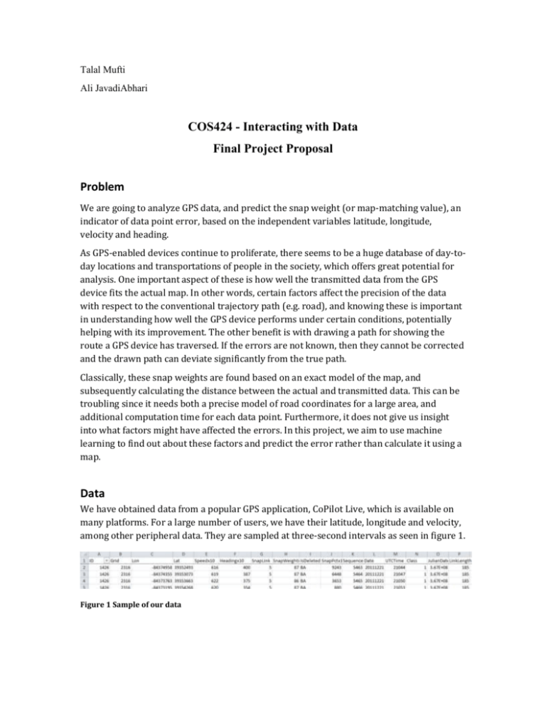
Talal Mufti
Ali JavadiAbhari
COS424 - Interacting with Data
Final Project Proposal
Problem
We are going to analyze GPS data, and predict the snap weight (or map-matching value), an
indicator of data point error, based on the independent variables latitude, longitude,
velocity and heading.
As GPS-enabled devices continue to proliferate, there seems to be a huge database of day-today locations and transportations of people in the society, which offers great potential for
analysis. One important aspect of these is how well the transmitted data from the GPS
device fits the actual map. In other words, certain factors affect the precision of the data
with respect to the conventional trajectory path (e.g. road), and knowing these is important
in understanding how well the GPS device performs under certain conditions, potentially
helping with its improvement. The other benefit is with drawing a path for showing the
route a GPS device has traversed. If the errors are not known, then they cannot be corrected
and the drawn path can deviate significantly from the true path.
Classically, these snap weights are found based on an exact model of the map, and
subsequently calculating the distance between the actual and transmitted data. This can be
troubling since it needs both a precise model of road coordinates for a large area, and
additional computation time for each data point. Furthermore, it does not give us insight
into what factors might have affected the errors. In this project, we aim to use machine
learning to find out about these factors and predict the error rather than calculate it using a
map.
Data
We have obtained data from a popular GPS application, CoPilot Live, which is available on
many platforms. For a large number of users, we have their latitude, longitude and velocity,
among other peripheral data. They are sampled at three-second intervals as seen in figure 1.
Figure 1 Sample of our data
In this dataset, we also have access to calculated snap-weights for each sample. The
company has developed a representation of the obtained values, shown in figure 2.
Methods
To predict snap weight from our independent variables, we propose experimenting with
several machine learning algorithms as well as different sets of assumptions. To begin we
take the case in which we assume our response variables to be independent and identically
distributed. This assumption, as well as the vocabulary of independent and dependent
variables lead us to begin our experiments with regression.
Though the odds of successfully modeling snap weight using a linear regression on a
function of position, speed, and heading are slim, we can also use these regressions to learn
more about the data by seeking patterns and ruling out our own hypotheses. Choosing
reasonable functions of the independent variables is a challenge as there seems to be no
literature on predicting snap weights without the use of the underlying GIS (graphical
information systems) data i.e. data for the location of the corresponding road.
Still our intuition says that significant and sudden deviations in speed, acceleration, or
heading are cause to believe a data point had a high margin of error – cars do not suddenly
pull an about-face. Similarly, roads are known to be constrained to certain curvatures to
reduce banking (inclining to one side of the vehicle due to angular momentum), therefore
sudden changes in heading can also be a potential indicator of an erroneous data point. A
regression line would capture this through deviation from the smooth line which we expect
when modeling speed or bearing. Should results look promising, we can then attempt to use
more advanced regression algorithms; least angle regression in particular seems appealing
as it is better at working with multiple potential covariates as we have here.
It is also reasonable to assume that since speed, heading, and even position can be
considered time-series (sequential) data, snap weight could possibly be modeled
sequentially as well, rather than as I.I.D. In our coursework so far we have only covered
Hidden Markov Models. Since we are currently most convinced by the variables speed and
heading, they can each be used as the observed variable for a separate HMM model. In both
cases, the hidden variable will of course be the snap weight that we seek.
In an attempt to capture a greater degree of complexity which HMMs cannot, we will then
look into more advanced models. A preliminary search led us to two potentially suitable
algorithms: Conditional Random Fields and Neural Networks, the latter of which was briefly
mentioned in our first reading. The goal here would be to look to consider not just the snap
weights as sequential data, but other variables as well.
Evaluation
The natural measure of evaluation is the average error percentage between the predicted
data and the dataset. We have a long vector of dependent variable data and the goal is to
minimize the average offset of the same column in our predicted values using either L1 or
L2 norms.
For evaluating how well we did in predicting the errors, we use a train/test/validation
approach. This means that we first hold out some of the data, called the test, and use the
remaining data to fit a model that is able to predict the snap weights. To be able to estimate
the parameters in this model, we can again use two sets: training and validation. Validation
data is used to tune the parameters we find using the training data. At the very end, to
evaluate our final model, we apply our model to the test data and measure the error we
encounter compared to the true data.
Contingency Plan
Should all of these methods fail to produce plausible predictors for the snap weight, it might
then be prudent to assume that it may be a function of the geographic location (see
clustering in figure 2). To test this however, we would require more data with a much
higher degree of spatial overlap. That is to say that for every arbitrarily assigned region (a
set of geographic points) we would require many data points all from that particular region.
Through this we can test to see if perhaps there are some intrinsic features of that region
which effect the GPS signal quality and therefore the snap value. For example a particular
region is near a factory and the smog affects the ionosphere or a dense forest canopy blocks
the GPS antennae of cars passing by there.
Figure 2 Snap Weight (snapValue) Representation