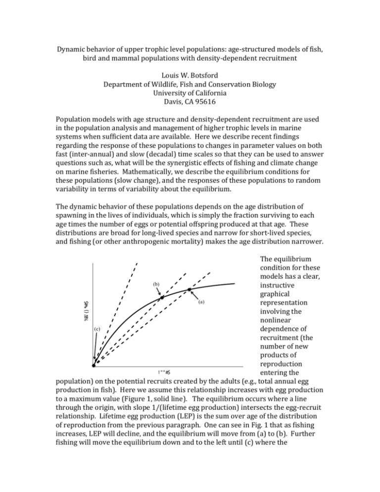
Dynamic behavior of upper trophic level populations: age-structured models of fish,
bird and mammal populations with density-dependent recruitment
Louis W. Botsford
Department of Wildlife, Fish and Conservation Biology
University of California
Davis, CA 95616
Population models with age structure and density-dependent recruitment are used
in the population analysis and management of higher trophic levels in marine
systems when sufficient data are available. Here we describe recent findings
regarding the response of these populations to changes in parameter values on both
fast (inter-annual) and slow (decadal) time scales so that they can be used to answer
questions such as, what will be the synergistic effects of fishing and climate change
on marine fisheries. Mathematically, we describe the equilibrium conditions for
these populations (slow change), and the responses of these populations to random
variability in terms of variability about the equilibrium.
The dynamic behavior of these populations depends on the age distribution of
spawning in the lives of individuals, which is simply the fraction surviving to each
age times the number of eggs or potential offspring produced at that age. These
distributions are broad for long-lived species and narrow for short-lived species,
and fishing (or other anthropogenic mortality) makes the age distribution narrower.
%&' () *+#$
The equilibrium
condition for these
models has a clear,
(b)
instructive
graphical
(a)
representation
involving the
nonlinear
(c)
dependence of
recruitment (the
number of new
products of
reproduction
! ""#$
entering the
population) on the potential recruits created by the adults (e.g., total annual egg
production in fish). Here we assume this relationship increases with egg production
to a maximum value (Figure 1, solid line). The equilibrium occurs where a line
through the origin, with slope 1/(lifetime egg production) intersects the egg-recruit
relationship. Lifetime egg production (LEP) is the sum over age of the distribution
of reproduction from the previous paragraph. One can see in Fig. 1 that as fishing
increases, LEP will decline, and the equilibrium will move from (a) to (b). Further
fishing will move the equilibrium down and to the left until (c) where the
equilibrium equals zero (i.e., the population will collapse). The way in which this
population equilibrium responds to fishing depends on the distribution of spawning
over age, which depends on survival and fecundity vs. age, both of which could
change with climate (slow time scale).
Inter-annual population variability is typically caused by inter-annual variability in
survival or fecundity at age, or inter-annual variability in development rate.
Variable survival and fecundity vary the magnitude of the spawning age distribution,
while variable development moves it back and forth between younger (fast
development) and older (slow development) age. The resulting population
variability can be observed in a time series of recruitment, egg production or catch.
The magnitudes of variability differ among these, but variability is generally
becomes greater as the slope at equilibrium of the egg-recruit function becomes
greater, i.e., as with fishing (Fig. 2a, b). This is the mechanism by which fishing a
population not only reduces recruitment and abundance, but also makes the
population more sensitive to environmental variability.
Changes in the shape of the spawning age distribution, either through fishing or
slow change in survival, fecundity or development rate also change the relative
sensitivity of a population to the frequencies of variability in the environment. The
bottom part of Fig. 2 illustrates the mechanism by which since the abundance at
each age depends on past values of recruitment, hence egg production forms a
positive feed-back of past values of recruitment on itself. In this mechanism, the
narrower the distribution of lags is, the greater the tendency is for the system to
resonate at a period equal to the mean lag, i.e., the generation time. Thus
populations are more sensitive to environmental variability on generational time
scales, more sensitive with narrower spawning age distributions, and less sensitive
with broader spawning age distributions. Populations are also more sensitive to
environmental variability on very slow time scales.
Figure 2. Schematic view of equilibrium and variability when unfished (a) and
fished (b).