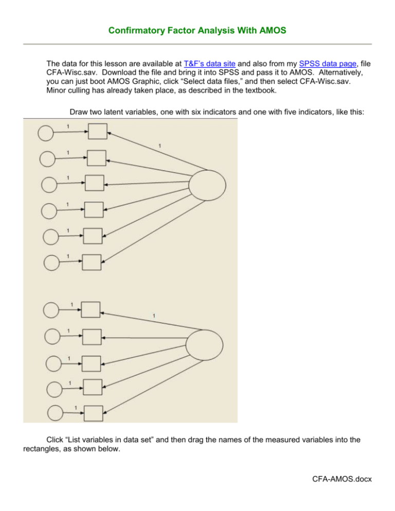
Confirmatory Factor Analysis With AMOS
The data for this lesson are available at T&F’s data site and also from my SPSS data page, file
CFA-Wisc.sav. Download the file and bring it into SPSS and pass it to AMOS. Alternatively,
you can just boot AMOS Graphic, click “Select data files,” and then select CFA-Wisc.sav.
Minor culling has already taken place, as described in the textbook.
Draw two latent variables, one with six indicators and one with five indicators, like this:
Click “List variables in data set” and then drag the names of the measured variables into the
rectangles, as shown below.
CFA-AMOS.docx
2
3
Using Object Properties, name the errors and factors, fix both factors to variance 1, remove
the fixed path coefficients, and draw a two-headed arrow like this:
4
Click “Analysis properties” and select the desired output:
Click “Calculate estimates.” Click “View the output path diagram” and “View Text.”
Look at the diagram with standardized estimates. Note that the solution is the same as that
shown in T & F Figure 14.10. The error variances for the measured variables, shown on the left in
Figure 14.10, are simply 1 minus the value of R2 shown in the Amos diagram. For example, for Info,
1 - .58 = .42.
Look at the text output. The null hypothesis of good fit is rejected, but this may be simply from
having too much power. The fit indices are OK. GFI (.931) exceeds .9, CFI (.941) does not quite
reach the .95 standard, and RMSEA (.06) is between good (.05) and adequate (.08).
The Standardized Residual Covariances are large for Comp-Pictcomp and Digit-Coding. The
Modification Indices for Covariances suggests linkage between e2 (error in comp) and Performance
IQ – perhaps we need a path from Performance IQ to Comp. The Modification Indices for Regression
Weights suggests linkage between Comp and (Object and Pictcomp), both of which are connected
with Performance IQ. Again, this suggests a path from Performance IQ to Comp. Let us add that
path and see what happens.
Diagram for Model 1.
5
6
Diagram for Model 2.
7
Look at the text output for the second model. The model fit Chi-square has dropped from
70.236 to 60.296, a drop of 9.94, which, on one df, is significant. Adding that path from Performance
IQ to Comp has significantly improved the fit of the model. GFI has increased from .931 to .942, CFI
from .941 to .960, and RMSEA has dropped from .06 to .05.
Notice that the path from Performance IQ to Coding is not statistically significant. Perhaps we
should just drop that variable. Drop it and see what happens.
With Coding out of the model, the goodness of fit Chi-square is no longer significant, 2(33) =
45.018, p = .079. GFI has increased from .94 to .952, CFI from .960 to .974, and RMSEA has
dropped from .05 to .046.
Links





CFA, including reliability and validity
Convert EFA to CFA
CFA Using AMOS – Indiana Univ.
CFA Using SAS Calis
Wuensch’s Stats Lessons
Karl L. Wuensch
Dept. of Psychology, East Carolina University, Greenville, NC 27858 USA
June, 2015