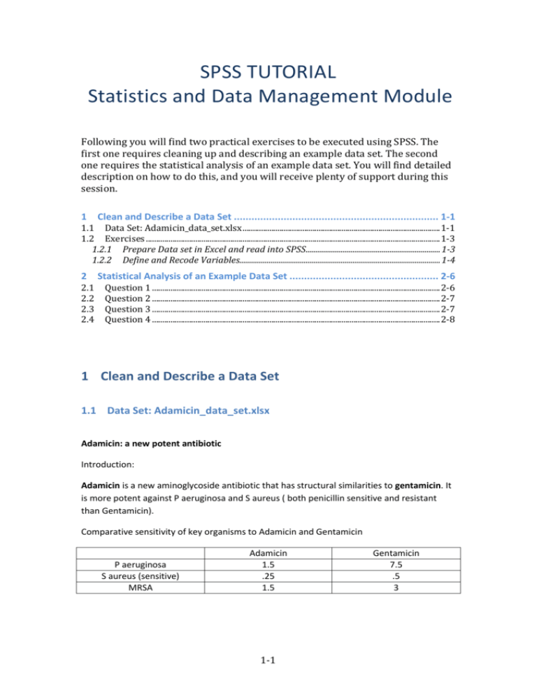
SPSS TUTORIAL
Statistics and Data Management Module
Following you will find two practical exercises to be executed using SPSS. The
first one requires cleaning up and describing an example data set. The second
one requires the statistical analysis of an example data set. You will find detailed
description on how to do this, and you will receive plenty of support during this
session.
1
Clean and Describe a Data Set ...................................................................... 1-1
1.1 Data Set: Adamicin_data_set.xlsx ................................................................................................ 1-1
1.2 Exercises ............................................................................................................................................... 1-3
1.2.1 Prepare Data set in Excel and read into SPSS..................................................................... 1-3
1.2.2 Define and Recode Variables....................................................................................................... 1-4
2
2.1
2.2
2.3
2.4
Statistical Analysis of an Example Data Set ................................................... 2-6
Question 1 ............................................................................................................................................ 2-6
Question 2 ............................................................................................................................................ 2-7
Question 3 ............................................................................................................................................ 2-7
Question 4 ............................................................................................................................................ 2-8
1 Clean and Describe a Data Set
1.1 Data Set: Adamicin_data_set.xlsx
Adamicin: a new potent antibiotic
Introduction:
Adamicin is a new aminoglycoside antibiotic that has structural similarities to gentamicin. It
is more potent against P aeruginosa and S aureus ( both penicillin sensitive and resistant
than Gentamicin).
Comparative sensitivity of key organisms to Adamicin and Gentamicin
P aeruginosa
S aureus (sensitive)
MRSA
Adamicin
1.5
.25
1.5
1-1
Gentamicin
7.5
.5
3
In animal studies Adamicin has been shown to be less nephrotoxic than Gentamicin. Other
nonclinical safety tests were unremarkable.
Adamicin is given by intravenous injection at a dose of 1.2 mg/kg per day in patients with
normal renal function. It has a Cmax of 14mg/l and a plasma half life of 15 hours. The trough
level is 3mg/l. Thus Adamicin can be given once a day as an IV bolus.
Gentamicin is also given by intravenous injection at a dose of 3 mg/kg per day in patients
with normal renal function. It has a Cmax of 20mg/l and a plasma half life of 4 hours. The
trough level is 2mg/l. Gentamicin is given as an IV bolus 3 times a day.
Both products have low binding to plasma proteins (30-35%) and are excreted largely
unchanged in the kidney.
They are both acid labile and therefore cannot be given by mouth.
Protocol:
Background: adults with cystic fibrosis usually have chronic infection in their lungs with P
aeruginosa, the colonisation starting in the early teenage years and proving almost
impossible to eliminate. In addition they often experience acute respiratory infections with S
aureus, both sensitive and resistant varieties. Treatment can often be given at home by
inserting a central venous line, but if the infection becomes too severe the patient will have
to be admitted to hospital.
Objective: this is a phase 2 open label study to compare Adamicin and Gentamicin in adults
with cystic fibrosis who have an acute respiratory infection with S. aureus.
Inclusion criteria: adult patients with cystic fibrosis have an acute respiratory infection
where the presumptive organism is thought to be S. aureus. The diagnosis of an acute
respiratory infection will be based on 2 of the following criteria:
a.
b.
c.
d.
Increased production of sputum
Change of colour of sputum
Fever - temperature more than 370 C
Increase in respiratory rate of more than 20% (Normal range 12 – 16 breaths
/minute)
e. Decrease in FEV1 of more than 10% (Normal range men aged 20 – 50 is 3.5 –
4.5L/sec and women 2.8 – 3.2 L/sec)
Exclusion criteria:
a. Patients who require immediate admission to hospital
b. Patients with any degree of renal impairment – BUN (Blood Urea Nitrogen) outside
normal range of 2.5-8.0 mmol/L
c. Patients with a history of hepatic or cardiac disease
d. Patients with cancer except non melanoma skin cancers
e. Patients who have had an acute respiratory infection within the past 4 weeks
1-2
Primary outcome measure: elimination of S.aureus at 14 days
Secondary outcome measures:
a.
b.
c.
d.
e.
Improvement in FEV1 (Forced Expiratory Volume 1)
Admission to hospital
Time off work/study
Change in renal function
Side effects
Design: This is an open label randomised study with a non-inferiority design, where the
hypothesis is that Adamicin is not inferior to Gentamicin. The inferiority margin is 10%. Only
patients who have a positive culture for S. aureus (either penicillin sensitive or resistant) will
go into the efficacy analysis.
Numbers: 100 patients per group
Procedures: adult patients with cystic fibrosis who suffer from episodes of acute respiratory
infection will be invited to participate in the study when they attend for routine outpatient
visits. After being given the opportunity to read the study information sheet and signing the
consent document they will be screened for the inclusion and exclusion criteria and if
suitable with be given packs of study drug.
Patients will be screened for the exclusion criteria and have base line measurements of renal
function (BUN), FEV1, sputum volume and colour
When they have an acute episode they will take a sample of sputum and send it to the
central laboratory. They will immediately start on study drug for 14 days. On day 14 ± 1 day
they will attend the hospital for follow up sputum test, BUN and FEV1.
1.2 Exercises
1.2.1 Prepare Data set in Excel and read into SPSS
Open and compare the following two Excel worksheets:


The original: Adamicin_data_set.xlsx
The Edited for analysis: Adamicin_data_set_edited.xlsx
The following changes have been made to give the data the right format:
-
Limited variable names to one row. Avoid names starting with numbers, or “/”,”.”
signs, or spaces.
Replaced text by numeric codes  explained codes in an additional sheet.
1-3
-
Replaced missing values by missing value code e.g. -99
Note: Remember, numeric codes are always preferable, and you should never mix strings
and numbers.
Read in coded data into SPSS:
Open SPSS.
FILE>OPEN>DATA
Under Format drop down menu, pick Excel.
 Select Adamicin_data_set_edited.xlsx
 Make sure you read in the right sheet .
 Select “Read variable names from the first row of data”
 Save .sav file
-
-
Look in the Window ‘Data View’ (Windows can be switched by pressing tabs at the
bottom of the screen). After the first analysis assignment SPSS opens an output file.
Use [Alt] [Tab] to switch between the dataset and output file.
Commands can be saved in the syntax screen by pressing <Paste> in the menus
(instead of <Run>). Parts of the syntax can be selected to be executed with ‘Run’.
Closing SPSS: after all the work you may want to externally save some files.
Check that variables names have been read in correctly
Check that you have the right number of cases (200)
Check that, under variable view, all variables have been read as numeric, except for
AEs.
Check that variables such as FEV1, BUN or temperature have been read with
decimals.
1.2.2 Define and Recode Variables
1.2.2.1 Define Variable Properties
DATA>DEFINE VARIABLE PROPERTIES
Transfer all variables into box “Variables to Scan”. Click Continue. For each variable:
- Provide a label that describes the variable.
- Choose measurement level : Scale (continuous), Ordinal, or Nominal (categorical).
For categorical values, provide value labels. E.g. For Gender, Value = 1 Label = ’Male’
Value = 2 Label = ‘Female’
Tip: See that there are variables measured twice, and you can simply copy the variable
properties from the first using the button <Copy Properties From Another Variable>.
1-4
1.2.2.2 Recode Variables
The background information of the study describes a number of variables for which there
are values within a normal range, and abnormal values. Some of them are part of the
inclusion/exclusion criteria:
- Respiratory rate: Normal range 12 – 16 breaths /minute
- FEV1: Normal range men aged 20 – 50 is 3.5 – 4.5L/sec and women 2.8 – 3.2 L/sec
- BUN: normal range of 2.5-8.0 mmol/L
- S.aureus: Positive = Sensitive or Resistant, Negative = Negative.
For two of these variables, at each time point:
- Inspect the distribution of the variable
- Create a new dichotomized variable for each of them normal vs. abnormal or
positive vs. negative. Remember! Use numeric codes, and then provide value labels.
- Count the number of patients with abnormal levels
In SPSS:
 Frequency distributions at: ANALYZE>DESCRIPTIVE STATISTICS>FREQUENCIES. You can
get a histogram under <charts>.
 To dichotomize: TRANSFORM>RECODE INTO DIFFERENT VARIABLES. Tips: 1) You can
recode all repeated measures of the same variable at once. 2) Use the <If…> button when
different cut-offs apply to different individuals, e.g. FEV1 cut-offs for men and women.
 Once dichotomized, you can inspect the changes in category between baseline and day
14 using crosstabs: ANALYZE>DESCRIPTIVE STATISTICS>CROSSTABS
Cut and paste the graphs and frequency tables that you consider relevant in a word
document, to help you elaborate your responses to this practical. Do not paste anything that
you do not understand. You will need to interpret properly every table and graphic in your
hand-in document.
1.2.2.3 Describe Variables
For the following variables: Gender, Age, BUNBaseline, FEV1Baseline, Baseline resp rate,
Sputum Vol, Sputum colour and Medication:
- Describe type of variable: independent vs. dependent, scale of measurement
(Categorical, Ordinal, Continuous).
- Use Descriptive statistics or frequency distributions as appropriate.
- Use graphs as appropriate, e.g. histograms or boxplots for continuous variables, bar
or pie charts for categorical variables.
- For Continuous variables, decide whether they are normally distributed, if they can
be analysed as continuous or rather grouped into ordinal categories, or
dichotomized.
- For categorical variables, decide whether there are sufficient number of patients in
each category or if some categories need to be merged.
In SPSS:
1-5
 Descriptive statistics: ANALYZE>DESCRIPTIVE STATISTICS>DESCRIPTIVES: This dialogue
provides basic descriptives only. ANALYZE>DESCRIPTIVE STATISTICS>EXPLORE: This dialogue
provides a larger list of statistics, as well as plots and normality tests. Descriptives can be
obtained for separate groups e.g. Medication, adding the grouping variable under “Factor
List”.
 Graphics: For GRAPHS>CHART BUILDER: Here you can make further graphics where
different groups are depicted in e.g. different boxplots. However, here only independent
groups can be depicted together in the same graphic. GRAPHS>LEGACY DIALOGS: here you
can depict paired samples within the same plot e.g. repeated measures of FEV1.
2 Statistical Analysis of an Example Data Set
Using the SPSS data set from the Adamicin trial (Adamicin.sav), we are going to carry
out a number of statistical tests to test a series of hypothesis and assumptions. Please,
consult your book and or lecture notes to decide the appropriate statistical test to apply
in each case.
Note: In some of the exercises you are required to test hypotheses regarding more than
one outcome variable, e.g. Sputum Volume and Temperature. Most of the statistical
techniques can be carried out simultaneously for several outcome variables. However,
only if you feel very confident and see that you progress at good rhythm, carry out
analysis for both; otherwise, proceed with only one of them. It is more important for you
to get to the end of the practical.
2.1 Question 1
When carrying out a clinical trial, it is important to test imbalances between groups in
relevant variables:
1. Are there any significant differences in Sputum Volume, or temperature at
baseline between the treatment groups i.e. Adamicin/Gentamicin?
a. Look at the distribution of the outcome variables (normality tests, mean
and median, skewness, qq-plots) to decide whether parametric or nonparametric statistics are appropriate for each test.
b. For each statistical test, phrase the null hypothesis, report the relevant
statistics, and produce the appropriate graphic to illustrate the results.
2. Using the dichotomized variables created yesterday, test for imbalances in
Baseline BUN and respiratory rate.
a. Obtain the appropriate statistic, phrase the null hypothesis, and
interpret the results using percentages and residuals.
b. Produce the appropriate graph to illustrate the results.
In SPSS:
 T-tests in ANALYZE>COMPARE MEANS
 Non-parametric tests in ANALYZE>NONPARAMETRIC TESTS
2-6
 Crosstabs (Chi-squared tests) in ANALYZE>DESCRIPTIVE STATISTICS>CROSSTABS
2.2 Question 2
Let’s look now at how a few of the secondary symptoms measured in the study changed
between entry and the 14 days after treatment, separately for the two treatment groups.
To carry out simultaneous, but independent analysis in two groups in the data
set, we need to split the data. In SPSS DATA>SPLIT FILE, select “compare groups”, and
add “Medication” in the <Groups Based on> box. Click <OK>.
1. Is there a decrease in Temperature or sputum volume between entry and 14
days after treatment in either of the treatment groups?
a. Decide and justify what is the appropriate statistical test.
b. For each test, phrase the null hypothesis, interpret the results and
illustrate them with the appropriate graphic.
2. Using the dichotomous variables, check whether there is a change in 1)
Respiratory rate between entry and 14 days; or 2) S. Aureus between baseline
and 14 days.
a. Obtain the appropriate statistic, phrase the null hypothesis, and
interpret the results using percentages and residuals.
b. Produce the appropriate graph to illustrate the results.
In SPSS:
 When you finish with this section, make sure that you un-split the file. DATA>SPLIT
FILE select <Analyze all cases, do not create groups>.
2.3 Question 3
We have seen that both treatment groups experience an improvement in temperature
and Sputum Volume between baseline and 14 days after treatment. What we need to
know is whether such improvement is better in the Adamicin group compared to the
Gentamicin group. Choose one of the two outcome variables for this exercise
(temperature or sputum volume), and test whether the two treatment groups differ in
temperature/sputum at 14 days after treatment, controlling for the baseline level.
In SPSS:
 Univariate ANOVA in ANALYZE> GENERAL LINEAR MODEL>UNIVARIATE.
 Tip: Treatment is the categorical independent variable of interests, and thus it is said
to have “fixed effects”. The baseline level of the continuous outcome variable is
something we want to control for, to avoid possible confounding due to imbalance at
baseline, and thus it is considered a “covariate”.
-
Phrase the null hypothesis
Interpret the results
Make a graph to represent the results.
2-7
2.4 Question 4
The final question we want to answer relates to the primary outcome, S Aureus
(dichotomized). Remember that this is a non-inferiority trial, with a non-inferiority limit
of 10%. The protocol stated: “adult patients with cystic fibrosis have an acute respiratory
infection where the presumptive organism is thought to be S. aureus”. Thus, for the
following analysis we need to select patients positive for S Aureus at entry.
 In SPSS, DATA>SELECT CASES> IF CONDITION IS SATISFIED. Define the condition as
S Aureus at entry = positive (resistant or sensitive).
1. Test whether the two treatment groups differ in the rate of positive S Aureus 14
days after treatment. Choose the right statistic to make a decision against the
null hypothesis. Interpret the results using percentages and residuals.
2-8