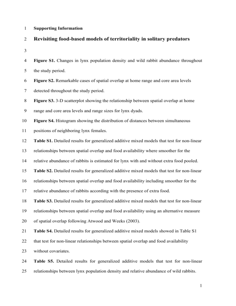
1
Supporting Information
2
Revisiting food-based models of territoriality in solitary predators
3
4
Figure S1. Changes in lynx population density and wild rabbit abundance throughout
5
the study period.
6
Figure S2. Remarkable cases of spatial overlap at home range and core area levels
7
detected throughout the study period.
8
Figure S3. 3-D scatterplot showing the relationship between spatial overlap at home
9
range and core area levels and range sizes for lynx dyads.
10
Figure S4. Histogram showing the distribution of distances between simultaneous
11
positions of neighboring lynx females.
12
Table S1. Detailed results for generalized additive mixed models that test for non-linear
13
relationships between spatial overlap and food availability where smoother for the
14
relative abundance of rabbits is estimated for lynx with and without extra food pooled.
15
Table S2. Detailed results for generalized additive mixed models that test for non-linear
16
relationships between spatial overlap and food availability including smoother for the
17
relative abundance of rabbits according with the presence of extra food.
18
Table S3. Detailed results for generalized additive mixed models that test for non-linear
19
relationships between spatial overlap and food availability using an alternative measure
20
of spatial overlap following Atwood and Weeks (2003).
21
Table S4. Detailed results for generalized additive mixed models showed in Table S1
22
that test for non-linear relationships between spatial overlap and food availability
23
without covariates.
24
Table S5. Detailed results for generalized additive models that test for non-linear
25
relationships between lynx population density and relative abundance of wild rabbits.
1
26
Figure S1. Changes in lynx population density (individuals 100 km-2; only sub-adult
27
and adult individuals, see text for details) and the relative abundance of wild rabbits
28
(rabbits km-1, see text for details) throughout the study period (note that both estimates
29
are only shown for those years with data on lynx spatial ecology. Circles denote records
30
of lynx population density in Vera (VE, black), and Coto del Rey (CR, grey). Upward
31
triangles refer to the annual maximum relative abundance of wild rabbits (between April
32
and July), whereas downward triangles refer to the annual minimum (between August
33
and November). Black triangles refers to VE and grey triangles to CR.
34
VE
CR
14
25
12
10
15
8
10
6
-1
20
4
5
2
0
1985
35
16
Wild rabbits km
-2
Lynx density (individuals 100 km )
30
0
1990
1995
2000
2005
2010
Year
36
37
2
38
Figure S2. Occasional cases of remarkable spatial overlap of home ranges (HR; 90%
39
probability contour of positions distribution) and core areas (CA, 50% probability
40
contour of positions distribution). Black boxes above the X-axis indicate years with
41
lynx data (12 years). Large grey open circles denote cases recorded between August and
42
November (i.e. low rabbit abundance period). The vertical dashed line separates cases
43
between areas (VE and CR). Shaded areas denote extraordinary events: the rabbit
44
population crash following the introduction of the rabbit haemorrhagic disease in 1990
45
(Moreno et al. 2007), a period of heavy rains (1995-1997) that further decimated the
46
rabbit population (Palomares 2003), and experimental supplementation of food between
47
2004 and 2008 (López-Bao, Rodríguez & Palomares 2008). The vertical white line
48
denotes the outbreak of the feline leukemia virus in CR in 2007, which led to the death
49
of 5 lynx in this area in a 6-month period (Meli et al. 2009).
HR overlap
CR
VE
CA overlap
0.6
Spatial overlap
0.5
0.4
0.3
0.2
0.1
1985
50
1990
1995
2000
2005
2010
Year
51
3
52
References
53
López-Bao, J.V., Rodríguez, A. & Palomares, F. (2008) Behavioural response of a
54
trophic specialist, the Iberian lynx, to supplementary food: patterns of food use and
55
implications for conservation. Biological Conservation, 141, 1857˗1867.
56
Meli, M.L., Cattori, V., Vargas, A., Martínez, F., López, G., Zorrilla, I., Muñoz, A.,
57
Palomares, F., López-Bao, J.V., Pastor, J., Tandon, R., Willi, B., Hofmann-Lehmann, R.
58
& Lutz, H. (2009) Feline leukemia virus and other pathogens as important threats to the
59
survival of the critically endangered Iberian Lynx (Lynx pardinus). PLOS ONE, 4,
60
e4744.
61
Moreno, S., Beltrán, J.F., Cotilla, I., Kuffner, B., Laffitte, R., Jordán, G., Ayala, J.,
62
Quintero, M.C., Jiménez, A., Castro, F., Cabezas, S. & Villafuerte, R. (2007) Long-term
63
decline of the European wild rabbit (Oryctolagus cuniculus) in south-western Spain.
64
Wildlife Research, 34, 652-658.
65
66
Palomares F. (2003) The negative impact of heavy rains on the abundance of a
Mediterranean population of European rabbits. Mammalian Biology, 68, 224–234.
67
68
69
70
71
72
73
74
75
76
4
77
Figure S3. 3-D scatterplot showing the relationship between spatial overlap of home
78
ranges (HR; 90% probability contour of positions distribution) and core areas (CA, 50%
79
probability contour of positions distribution) and range sizes (HR and CA) for dyads of
80
neighbouring lynx (individuals A and B).
0.6
0.5
0.4
HR overlap
0.3
0.2
0.1
0.0
70
60
50
40
30
20
2
10
10
Home range A (km )
15
20
Home range B (km2)
5
0
35
30
25
0
0.25
0.20
0.15
CA overlap
0.10
0.05
0.00
14
12
10
8
2
81
Core Area A (km )
6
4
2
0
0
2
4
6
8
18
16
14
12
10
Core area B (km2)
82
83
84
5
85
Figure S4. Histogram showing the distribution of distances between simultaneous
86
positions of neighboring lynx females (500 m intervals). Grey bar: 0 - 500 m interval.
87
88
89
90
91
92
93
94
95
96
97
98
6
99
Table S1. Parameter estimates (± SE) in the generalized additive mixed models that test
100
for non-linear relationships between spatial overlap and food availability. A smoother
101
for the relative abundance of wild rabbits (rabbit availability) is estimated for lynx with
102
and without extra food pooled. The levels “extra food (absence)” and “area (VE)” are
103
included in the intercept. BIC = Bayesian Information Criterion. BIC tends to be more
104
conservative and less prone to over-parameterization than Akaike’s information
105
criterion (Bolker 2008).
Home range
estimate SE
Parametric coefficients:
Intercept
Extra food (presence)
Area (CR)
Radio-tracking effort
0.75
0.12
-0.41
-0.01
0.207
0.074
0.102
1
3.08
BIC = 42.46
P
0.001
0.21
0.09
0.22
0.01
Smooth terms:
ƒ (rabbit availability)
ƒ (lynx density)
106
107
edf
Core area
estimate SE
0.22
-0.07
-0.05
-0.01
edf
0.050
0.11
0.04
0.07
0.01
0.603
0.036
P
0.175
0.450
0.108
1
2.86
0.742
0.104
BIC = 6.68
edf = estimated degrees of freedom
108
109
110
111
References
Bolker, B.M. (2008) Ecological Models and Data in R. Princeton University Press,
Princeton, NJ, USA.
112
113
114
115
116
7
117
Table S2. Parameter estimates (± SE) in the alternative generalized additive mixed
118
models that test for non-linear relationships between spatial overlap and food
119
availability including smoothers for the relative abundance of wild rabbits during
120
periods with and without extra food. The levels “extra food (absence)” and “area (VE)”
121
are included in the intercept. BIC = Bayesian Information Criterion.
Home range
Parametric coefficients:
Intercept
Extra food (presence)
Area (CR)
Radio-tracking effort
estimate
SE
0.76
0.12
-0.41
-0.01
0.22
0.10
0.22
0.01
Smooth terms:
ƒ (rabbit availability) x absence
of extra food
ƒ (rabbit availability) x presence
of extra food
ƒ (lynx density)
BIC = 53.11
122
123
edf
Core area
P
0.001
0.246
0.075
0.127
estimate SE
0.13
-0.05
-0.01
-0.01
edf
0.10
0.05
0.08
0.01
P
0.230
0.362
0.856
0.478
1
0.731
3.22
0.133
1
0.647
1.77
0.413
3.05
0.029
2.36
0.026
BIC = 13.29
edf = estimated degrees of freedom
124
125
126
127
128
129
130
131
8
132
Table S3. Parameter estimates (± SE) in the generalized additive mixed models that test
133
for non-linear relationships between spatial overlap and food availability using an
134
alternative measure of spatial overlap proposed by Atwood and Weeks (2003). Based on
135
the size of adaptive kernel estimates of lynx home ranges (HR, 90% probability contour
136
of positions distribution) and core areas (CA, 50% probability contour of positions
137
distribution), spatial overlap indices were calculated as follow:
138
Overlap index = [(areaAB/sizeA) x (areaAB/sizeB)]0.5
139
where areaAB is the area shared (overlapped) at either HR or CA level, and sizeA and
140
sizeB are the individual sizes of HR or CA, respectively. Overlapped areas and the size
141
of HR and CA were calculated using ArcGIS 9 (ESRI, California, USA). Modeling
142
procedures and factors are explained in the methods section. The levels “extra food
143
(absence)” and “area (VE)” are included in the intercept.
Home range
Parametric coefficients:
Intercept
Extra food (presence)
Area (CR)
Radio-tracking effort
estimate
SE
0.76
0.16
-0.50
-0.01
0.18
0.09
0.19
0.01
Smooth terms:
ƒ (rabbit availability)
ƒ (lynx density)
144
edf
Core area
P
0.001
0.085
0.013
0.545
1.27
4.50
0.235
0.001
estimate SE
0.19
0.03
-0.16
-0.01
edf
0.14
0.07
0.11
0.01
P
0.176
0.610
0.142
0.852
1
2.93
0.235
0.044
edf = estimated degrees of freedom
145
146
References
147
Atwood, T.C. & Weeks, H.P. (2003) Spatial home-range overlap and temporal
148
interaction in eastern coyotes: The influence of pair types and fragmentation. Canadian
149
Journal of Zoology, 81, 1589-1597.
9
150
Table S4. Parameter estimates (± SE) in the generalized additive mixed models that test
151
for non-linear relationships between spatial overlap and food availability (see Table S1)
152
without covariates (area, lynx population density, radio-tracking effort). A smoother for
153
the relative abundance of wild rabbits (rabbit availability) is estimated for lynx with and
154
without extra food pooled. The level “extra food (absence)” is included in the intercept.
Home range
estimate SE
Parametric coefficients:
Intercept
Extra food (presence)
Smooth terms:
ƒ (rabbit availability)
155
156
0.30
0.12
edf
Core area
P
0.001
0.08
0.10
0.238
1.41
0.783
estimate SE
0.07
-0.05
edf
P
0.100
0.04
0.05
0.314
1
0.559
edf = estimated degrees of freedom
157
158
159
160
161
162
163
164
165
166
167
168
169
10
170
Table S5. Detailed results of four generalized additive models that test for non-linear
171
relationships between lynx population density (individuals 100 km-2; only sub-adult and
172
adult individuals, see text for details) and four estimates of the relative abundance of
173
wild rabbits (rabbits km-1, denoted as "WRA" in the table) throughout the study period
174
in VE and CR (total number of areas*year = 14). We tested four different estimates of
175
relative abundance of wild rabbits: the maximum (spring) and minimum (autumn)
176
values of wild rabbit abundance the same year, and the year before, that lynx population
177
density was recorded. We considered the maximum and the minimum values of rabbit
178
availability because they are proxies of two population processes affecting lynx density:
179
Productivity may be associated with prey availability in spring, whereas survival may
180
be associated with prey availability in autumn. The year before was considered to
181
explore the influence of time-delayed effects of prey availability on lynx population
182
density. The presence/absence of extra food and the area were considered as covariates
183
in all models.
184
MODEL considering:
Parametric coefficients:
Extra food
Area
Smooth terms:
ƒ (WRA)
185
186
Maximum WRA
the same year
F
df
2.22
32.3
1
1
P
Minimum WRA
the same year
F
0.117 2.26
0.001 26.6
edf
0.07
1
df
1
1
P
Maximum WRA
the year before
F
0.164 1.72
0.001 26.9
1
1
1
P
F
0.219 3.56
0.001 35.3
edf
edf
0.799 0.01
df
Minimum WRA
the year before
0.977 0.88
1
df
P
1
1
0.105
0.001
edf
0.369 2.97
3.6
edf = estimated degrees of freedom
11
0.107