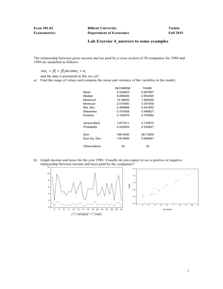
Econ 301.02
Econometrics
Bilkent University
Department of Economics
Taskin
Fall 2015
Lab Exercise 4_answers to some examples
The relationship between gross income and tax paid by a cross section of 30 companies for 1988 and
1989 are modelled as follows:
taxt  1   2incomet  ut
a)
and the data is presented in file tax.wf1
Find the range of values and compute the mean and variance of the variables in the model,
INCOME88
5.534833
5.095000
10.39400
2.015000
2.466989
0.375408
2.120476
TAX88
0.957667
0.853000
1.902000
0.351000
0.441652
0.499827
2.163562
Jarque-Bera
Probability
1.671611
0.433525
2.123670
0.345821
Sum
Sum Sq. Dev.
166.0450
176.4950
28.73000
5.656651
Observations
30
30
Mean
Median
Maximum
Minimum
Std. Dev.
Skewness
Kurtosis
b) Graph income and taxes for the year 1988. Visually do you expect to see a positive or negative
relationship between income and taxes paid by the companies?
12
2.0
10
1.6
8
TAX88
1.2
6
0.8
4
0.4
2
0.0
1
2
3
4
5
6
7
8
9
10
0
2
4
6
8
10
12
14
16
INCOME88
18
20
22
24
26
28
30
INCOME88
TAX88
1
11
c)
Estimate the above tax function for the year 1988.
Dependent Variable: TAX88
Method: Least Squares
Date: 10/05/05 Time: 05:45
Sample: 1 30
Included observations: 30
Variable
Coefficient
Std. Error
t-Statistic
Prob.
C
INCOME88
-0.018003
0.176278
0.035678
0.005904
-0.504586
29.85734
0.6178
0.0000
R-squared
Adjusted R-squared
S.E. of regression
Sum squared resid
Log likelihood
Durbin-Watson stat
0.969547
0.968460
0.078436
0.172260
34.83107
2.442251
Mean dependent var
S.D. dependent var
Akaike info criterion
Schwarz criterion
F-statistic
Prob(F-statistic)
0.957667
0.441652
-5.026615
-4.933202
891.4607
0.000000
d) The fitted (estimated) tax relationship for 1988. Compute the fitted values of taxes.
taˆxt  ˆ1  ˆ2incomet
taˆxt  0.018  0.176incomet
e)
The plot (graph) of the actual, fitted values of taxes for 30 companies and the residual
values. Which company’s tax value is explained the best and which one’s tax values are
explained the worst by the estimated equation? What are special for these observations?
(What are the stylized facts?)
f)
The sum of squared residuals=0.172260 and R2=0.9695 of the regression
2
g) The estimated unbiased variance of the error term, ie. ˆ =(0.078436)2
h) The 95% confidence interval for the marginal tax rate , b̂ 2 .
Pr éëb̂2 - ŝ b̂ .ta /2,d. f . £ b2 £ b̂2 + ŝ b̂ .ta /2,d. f . ùû =1- a
2
2
Pr0.176  (0.0059)(2.048)  2  0.176  (0.0059).(2.048)  1  0.05
Pr0.176  (0.01208)  2  0.176  (0.01208)  1  0.05
Pr0.1639  2  0.1881  0.95
i)
Test the following hypothesis
H o :   0.2
H A :   0.2
at the 5% significance level.
The test statistic which has a student’s t distribution is
t _ stat 
ˆ 2   2
ˆ ˆ
2
This test statistic will have the
t _ stat 
ˆ2  0.2 0.176  0.2

 4.065 value.
ˆ ˆ
0.005904
2
If the null hypothesis is supported by the sample data then this test statistic ie. t-stat should conform to
a t-distribution. This means that
2


Pr t / 2,d . f .  t _ stat  t / 2,d . f .  1  
So we need to check whether this in fact is true. Is t-stat follows the below inequality;
Pr2.048  t _ stat  2.048  0.95
The answer is NO, since it is not in the t_stat interval. Hence we can reject the null hypothesis
j)
Test the significance of the income variable.
Ho : b = 0
HA : b ¹ 0
For this null hypothesis
t  stat 
ˆ2
0.176

 29.857 . If this
ˆ ˆ
0.005904
t-stat conform to the
2
below inequality then we can not reject the null hypothesis.


Pr t / 2,d . f .  t _ stat  t / 2,d . f .  1   or Pr2.048  29.857  2.048  0.95
The interpretation is that is unlikely that the sample is drawn from a population with the
Hence, Income is a statistically significant variable in explaining the tax values.
b̂2 = 0.0 .
(Note: Student’s t value for 0.025 significance level and 28 degrees of freedom (n-2) is equal to
2.048)
3