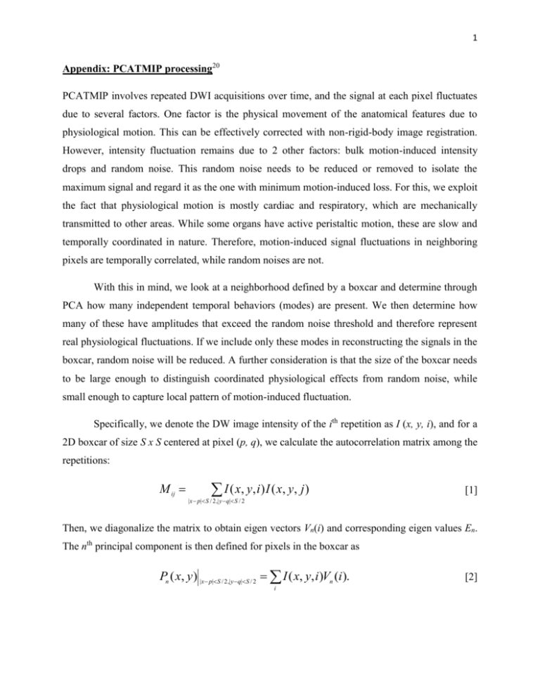
1
Appendix: PCATMIP processing20
PCATMIP involves repeated DWI acquisitions over time, and the signal at each pixel fluctuates
due to several factors. One factor is the physical movement of the anatomical features due to
physiological motion. This can be effectively corrected with non-rigid-body image registration.
However, intensity fluctuation remains due to 2 other factors: bulk motion-induced intensity
drops and random noise. This random noise needs to be reduced or removed to isolate the
maximum signal and regard it as the one with minimum motion-induced loss. For this, we exploit
the fact that physiological motion is mostly cardiac and respiratory, which are mechanically
transmitted to other areas. While some organs have active peristaltic motion, these are slow and
temporally coordinated in nature. Therefore, motion-induced signal fluctuations in neighboring
pixels are temporally correlated, while random noises are not.
With this in mind, we look at a neighborhood defined by a boxcar and determine through
PCA how many independent temporal behaviors (modes) are present. We then determine how
many of these have amplitudes that exceed the random noise threshold and therefore represent
real physiological fluctuations. If we include only these modes in reconstructing the signals in the
boxcar, random noise will be reduced. A further consideration is that the size of the boxcar needs
to be large enough to distinguish coordinated physiological effects from random noise, while
small enough to capture local pattern of motion-induced fluctuation.
Specifically, we denote the DW image intensity of the ith repetition as I (x, y, i), and for a
2D boxcar of size S x S centered at pixel (p, q), we calculate the autocorrelation matrix among the
repetitions:
M ij 
 I ( x, y , i ) I ( x, y , j )
[1]
|x  p| S / 2 ,| y  q| S / 2
Then, we diagonalize the matrix to obtain eigen vectors Vn(i) and corresponding eigen values En.
The nth principal component is then defined for pixels in the boxcar as
Pn ( x, y ) |x p|S / 2,| y q|S / 2   I ( x, y, i )Vn (i ).
i
[2]
2
Next, we select the PCs corresponding to eigenvalues above a threshold Et and reconstruct PCAfiltered intensity values in the box using these principal components:
'
 x, y , i  x  p  S / 2 , y  q  S / 2 
I pq
 P x, y V i 
En  Et
n
n
[3]
This process is repeated through a sliding box process in which the center (p, q) of the boxcar is
moved over the entire image at 1 pixel increments. In doing so, each pixel (x, y) is covered by
many boxcars, and each boxcar generates a set of filtered intensities I’pq(x,y,i). At each pixel,
these boxcars are combined in a weighted sum to yield the final PCA filtered image intensity for
pixel (x, y) and the ith repetition:
'
 x, y , i 
I PCA x, y, i    wx  p, y  q  I pq
[4]
p ,q
where the weight w decreases with increasing distance between (x, y) and (p, q).
The 2 key parameters in the PCA process are the size of the sliding boxcar S and the
eigenvalue threshold Et. As indicated earlier, the size of the boxcar needs to be large enough to
distinguish coordinated physiological effects from random noise and small enough to capture the
local pattern of motion-induced fluctuation. Thus, the box size should be small enough that no
more than 2 compartments are included; thus, 2 PCs are needed to describe the intensity
fluctuations in the box, but large enough so that the error in the PCA filtered intensity approaches
the theoretical level of:
Error in PCA filtered intensity 
number of included PCs
 ( noise level in a single image)
number of repetition s
[5]
The eigenvalue threshold Et should be set high enough to reject the PCs corresponding to pixelwise random noise and low enough to include the PCs from global intensity fluctuations caused
by motion. Both parameters were determined by numerical simulations based on the SNR level of
experimentally acquired DW images. Based on the observed SNR in our volunteers, the optimal
box size was determined to be 15 x 15 pixels and the optimal threshold Et = 40*<E>3 to 10.
In the last step, the PCA-filtered images were then subjected to TMIP to yield a single
DW image for each diffusion weighting and gradient direction:
3
I PCATMIP ( x, y )  ( MIP along repetition i )I PCA ( x, y , i )
[6]
Figure A. Block diagram of PCATMIP processing flow. Blocks represent processing steps; input,
intermediate results and outputs are shown in bold. Transferred data are symbolized by arrows
connecting blocks.