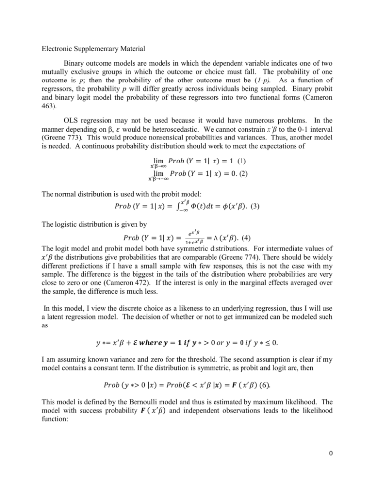
Electronic Supplementary Material
Binary outcome models are models in which the dependent variable indicates one of two
mutually exclusive groups in which the outcome or choice must fall. The probability of one
outcome is p; then the probability of the other outcome must be (1-p). As a function of
regressors, the probability p will differ greatly across individuals being sampled. Binary probit
and binary logit model the probability of these regressors into two functional forms (Cameron
463).
OLS regression may not be used because it would have numerous problems. In the
manner depending on β, 𝜀 would be heteroscedastic. We cannot constrain x’β to the 0-1 interval
(Greene 773). This would produce nonsensical probabilities and variances. Thus, another model
is needed. A continuous probability distribution should work to meet the expectations of
lim 𝑃𝑟𝑜𝑏 (𝑌 = 1| 𝑥) = 1 (1)
x’β→∞
lim 𝑃𝑟𝑜𝑏 (𝑌 = 1| 𝑥) = 0. (2)
x’β→−∞
The normal distribution is used with the probit model:
𝑥′𝛽
𝑃𝑟𝑜𝑏 (𝑌 = 1| 𝑥) = ∫−∞ 𝛷(𝑡)𝑑𝑡 = 𝜙(𝑥 ′ 𝛽). (3)
The logistic distribution is given by
′
𝑒𝑥 𝛽
𝑃𝑟𝑜𝑏 (𝑌 = 1| 𝑥) =
= ∧ (𝑥 ′ 𝛽). (4)
′
1+𝑒 𝑥 𝛽
The logit model and probit model both have symmetric distributions. For intermediate values of
𝑥 ′ 𝛽 the distributions give probabilities that are comparable (Greene 774). There should be widely
different predictions if I have a small sample with few responses, this is not the case with my
sample. The difference is the biggest in the tails of the distribution where probabilities are very
close to zero or one (Cameron 472). If the interest is only in the marginal effects averaged over
the sample, the difference is much less.
In this model, I view the discrete choice as a likeness to an underlying regression, thus I will use
a latent regression model. The decision of whether or not to get immunized can be modeled such
as
𝑦 ∗= 𝑥 ′ 𝛽 + 𝓔 𝒘𝒉𝒆𝒓𝒆 𝒚 = 𝟏 𝒊𝒇 𝒚 ∗ > 0 𝑜𝑟 𝑦 = 0 𝑖𝑓 𝑦 ∗ ≤ 0.
I am assuming known variance and zero for the threshold. The second assumption is clear if my
model contains a constant term. If the distribution is symmetric, as probit and logit are, then
𝑃𝑟𝑜𝑏 (𝑦 ∗> 0 |𝑥) = 𝑃𝑟𝑜𝑏(𝓔 < 𝑥 ′ 𝛽 |𝒙) = 𝑭 ( 𝑥 ′ 𝛽) (6).
This model is defined by the Bernoulli model and thus is estimated by maximum likelihood. The
model with success probability 𝑭 ( 𝑥 ′ 𝛽) and independent observations leads to the likelihood
function:
0
𝑃𝑟𝑜𝑏 (𝑌1 = 𝑦1, 𝑌2 = 𝑦2, … . , 𝑌𝑛 = 𝑦𝑛 |X) = ∏[1 − 𝑭 ( 𝑥𝑖 ′ 𝛽) ] ∏ 𝑭 ( 𝑥𝑖 ′ 𝛽).
𝑦𝑖 =0
𝑦𝑖 =1
The likelihood function for n observations can be written as
𝑛
𝐿(𝛽 |𝑑𝑎𝑡𝑎) = ∏[𝑭 ( 𝑥𝑖 ′ 𝛽)]𝑦𝑖 [1 − 𝑭 ( 𝑥𝑖 ′ 𝛽)]1−𝑦𝑖
𝑖=1
After taking logs,
𝑛
ln 𝐿 = ∑{𝑦𝑖 ln 𝑭 ( 𝑥𝑖 ′ 𝛽) + (1 − 𝑦𝑖 ) ln [1 − 𝑭 ( 𝑥𝑖 ′ 𝛽)]}.
𝑖=1
The likelihood equations are
𝑛
𝑑𝑙𝑛 𝐿
𝑦𝑖 𝑓𝑖
– 𝑓𝑖
= ∑[
+ (1 − 𝑦𝑖 )
] 𝑥 = 0.
(1 − 𝐹𝑖 ) 𝑖
𝑑𝛽
𝐹𝑖
𝑖=1
The density is 𝑓𝑖 .
For the logit model, the first order conditions are
𝑛
𝑑𝑙𝑛 𝐿
= ∑( 𝑦𝑖 −∧)𝑥𝑖 = 0.
𝑑𝛽
𝑖=1
The second derivatives for the logit model are:
𝑯 = − ∑𝑖 ∧𝑖 (1 − ∧𝑖 )𝒙𝑖 𝒙𝑖 ′.
Newton’s method of scoring can be used since the random variable 𝑦𝑖 is not included in the
second derivatives for the logit model. The log-likelihood is globally concave and this method
will normally converge to the log-likelihood maximum in minimal iterations (Greene 779).
My interest is in determining the marginal effect of a change in the regressor on the conditional
probability that y is equal to one. Typical binary outcome models are single-index, which allow
the ratio of coefficients for two regressors to equal the ratio of the marginal effects. The sign of
the marginal effect is given by the sign of the coefficient (Cameron 469). The marginal effects of
the logit model can be obtained from the coefficients, with
𝑑𝑝𝑖
= 𝑝𝑖 (1 − 𝑝𝑖 ), 𝑤ℎ𝑒𝑟𝑒 𝑝𝑖 = ⋀𝑖 = ⋀(𝐱 ′ 𝛃).
𝑑𝑥𝑖𝑗
Interpreting the coefficients is frequently done in terms of the marginal effects on the odds
ratio. For the logit model:
𝑝 = exp( 𝒙′ 𝛽)/(1 + exp(𝒙′ 𝛽)
Which implies
ln
𝑝
= 𝒙′ 𝛽.
1−𝑝
1
The odds ratio, or relative risk measures the probability of y being equal to one in relation to the
probability of y being equal to zero, this is p/(1-p). The log-odds ratio is linear for the logit model
(Cameron 470).
All calculations were performed using SAS.
Number of Observations
Hosmer and Lemeshow
Goodnes of Fit Test
Likelihood Ratio
Score
Wald
14,951
Chi-Square
Pr > ChiSq
2.943
58.34
55.09
49.29
0.1409
<.0001
<.0001
<.0001
2