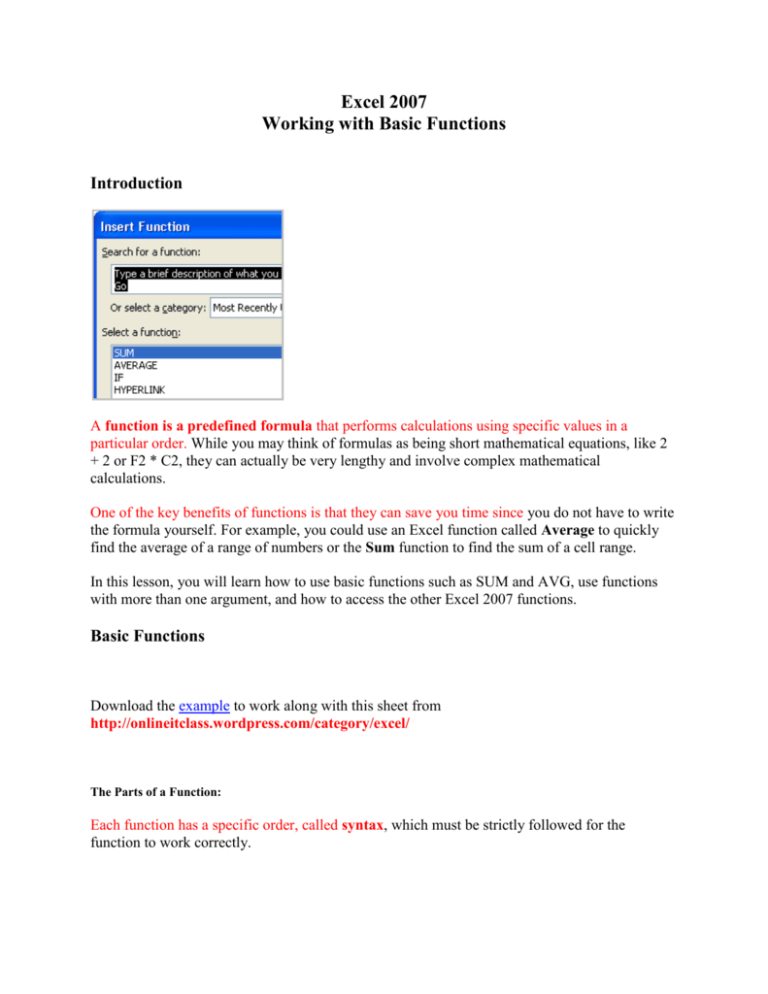
Excel 2007
Working with Basic Functions
Introduction
A function is a predefined formula that performs calculations using specific values in a
particular order. While you may think of formulas as being short mathematical equations, like 2
+ 2 or F2 * C2, they can actually be very lengthy and involve complex mathematical
calculations.
One of the key benefits of functions is that they can save you time since you do not have to write
the formula yourself. For example, you could use an Excel function called Average to quickly
find the average of a range of numbers or the Sum function to find the sum of a cell range.
In this lesson, you will learn how to use basic functions such as SUM and AVG, use functions
with more than one argument, and how to access the other Excel 2007 functions.
Basic Functions
Download the example to work along with this sheet from
http://onlineitclass.wordpress.com/category/excel/
The Parts of a Function:
Each function has a specific order, called syntax, which must be strictly followed for the
function to work correctly.
Syntax Order:
1. All functions begin with the = sign.
2. After the = sign define the function name (e.g., Sum).
3. Then there will be an argument. An argument is the cell range or cell references that are
enclosed by parentheses. If there is more than one argument, separate each by a comma.
An example of a function with one argument that adds a range of cells, A3 through A9:
An example of a function with more than one argument that calculates the sum of two cell
ranges:
Excel literally has hundreds of different functions to assist with your calculations. Building
formulas can be difficult and time-consuming. Excel's functions can save you a lot of time and
headaches.
Excel's Different Functions
There are many different functions in Excel 2007. Some of the more common functions include:
Statistical Functions:





SUM - summation adds a range of cells together.
AVERAGE - average calculates the average of a range of cells.
COUNT - counts the number of chosen data in a range of cells.
MAX - identifies the largest number in a range of cells.
MIN - identifies the smallest number in a range of cells.
Financial Functions:



Interest Rates
Loan Payments
Depreciation Amounts
Date and Time functions:









DATE - Converts a serial number to a day of the month
Day of Week
DAYS360 - Calculates the number of days between two dates based on a 360-day year
TIME - Returns the serial number of a particular time
HOUR - Converts a serial number to an hour
MINUTE - Converts a serial number to a minute
TODAY - Returns the serial number of today's date
MONTH - Converts a serial number to a month
YEAR - Converts a serial number to a year
You don't have to memorize the functions but should have an idea of what each can do for you.
To Calculate the Sum of a Range of Data Using AutoSum:





Select the Formulas tab.
Locate the Function Library group. From here, you can access all the available
functions.
Select the cell where you want the function to appear. In this example, select G42.
Select the drop-down arrow next to the AutoSum command.
Select Sum. A formula will appear in the selected cell, G42.
o This formula, =SUM(G2:G41), is called a function. AutoSum command
automatically selects the range of cells from G2 to G41, based on where you
inserted the function. You can alter the cell range, if necessary.

Press the Enter key or Enter button on the formula bar. The total will appear.
To Edit a Function:



Select the cell where the function is defined.
Insert the cursor in the formula bar.
Edit the range by deleting and changing necessary cell numbers.

Click the Enter icon.
To Calculate the Sum of Two Arguments:



Select the cell where you want the function to appear. In this example, G44.
Click the Insert Function command on the Formulas tab. A dialog box appears.
SUM is selected by default.




Click OK and the Function Arguments dialog box appears so that you can enter the
range of cells for the function.
Insert the cursor in the Number 1 field.
In the spreadsheet, select the first range of cells. In this example, G21 through G26. The
argument appears in the Number 1 field.
o To select the cells, left-click cell G21 and drag the cursor to G26, and then
release the mouse button.
Insert the cursor in the Number 2 field.



In the spreadsheet, select the second range of cells. In this example, G40 through G41.
The argument appears in the Number 2 field.
Notice that both arguments appear in the function in cell G44 and the formula bar when
G44 is selected.
Click OK in the dialog box and the sum of the two ranges is calculated.
To Calculate the Average of a Range of Data:


Select the cell where you want the function to appear.
Click the drop-down arrow next to the AutoSum command.




Select Average.
Click on the first cell (in this example, C8) to be included in the formula.
Left-click and drag the mouse to define a cell range (C8 through cell C20, in this
example).
Click the Enter icon to calculate the average.
Accessing Excel 2007 Functions
To Access Other Functions in Excel:





Using the point-click-drag method, select a cell range to be included in the formula.
On the Formulas tab, click on the drop-down part of the AutoSum button.
If you don't see the function you want to use (Sum, Average, Count, Max, Min), display
additional functions by selecting More Functions.
The Insert Function dialog box opens.
There are three ways to locate a function in the Insert Function dialog box:
You can type a question in the Search for a function box and click GO, or
You can scroll through the alphabetical list of functions in the Select a function field, or
You can select a function category in the Select a category drop-down list and review the
corresponding function names in the Select a function field.

Select the function you want to use and then click the OK button.
Challenge!
Use the Inventory workbook or any workbook you choose to complete this challenge.



Use a SUM function to calculate the sum of one argument.
Use the AVG function to calculate the sum of a range of cells.
Explore the other Excel 2007 functions.