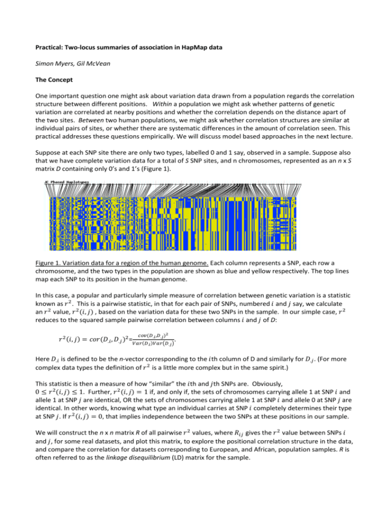
Practical: Two-locus summaries of association in HapMap data
Simon Myers, Gil McVean
The Concept
One important question one might ask about variation data drawn from a population regards the correlation
structure between different positions. Within a population we might ask whether patterns of genetic
variation are correlated at nearby positions and whether the correlation depends on the distance apart of
the two sites. Between two human populations, we might ask whether correlation structures are similar at
individual pairs of sites, or whether there are systematic differences in the amount of correlation seen. This
practical addresses these questions empirically. We will discuss model based approaches in the next lecture.
Suppose at each SNP site there are only two types, labelled 0 and 1 say, observed in a sample. Suppose also
that we have complete variation data for a total of S SNP sites, and n chromosomes, represented as an n x S
matrix D containing only 0’s and 1’s (Figure 1).
Figure 1. Variation data for a region of the human genome. Each column represents a SNP, each row a
chromosome, and the two types in the population are shown as blue and yellow respectively. The top lines
map each SNP to its position in the human genome.
In this case, a popular and particularly simple measure of correlation between genetic variation is a statistic
known as 𝑟 2 . This is a pairwise statistic, in that for each pair of SNPs, numbered 𝑖 and 𝑗 say, we calculate
an 𝑟 2 value, 𝑟 2 (𝑖, 𝑗) , based on the variation data for these two SNPs in the sample. In our simple case, 𝑟 2
reduces to the squared sample pairwise correlation between columns 𝑖 and 𝑗 of D:
𝑐𝑜𝑣(𝐷.𝑖 ,𝐷.𝑗 )2
𝑟 2 (𝑖, 𝑗) = 𝑐𝑜𝑟(𝐷.𝑖 , 𝐷.𝑗 )2 =𝑉𝑎𝑟(𝐷
.
.𝑖 )𝑉𝑎𝑟(𝐷.𝑗 )
Here 𝐷.𝑖 is defined to be the n-vector corresponding to the 𝑖th column of D and similarly for 𝐷.𝑗 . (For more
complex data types the definition of 𝑟 2 is a little more complex but in the same spirit.)
This statistic is then a measure of how “similar” the 𝑖th and 𝑗th SNPs are. Obviously,
0 ≤ 𝑟 2 (𝑖, 𝑗) ≤ 1. Further, 𝑟 2 (𝑖, 𝑗) = 1 if, and only if, the sets of chromosomes carrying allele 1 at SNP 𝑖 and
allele 1 at SNP 𝑗 are identical, OR the sets of chromosomes carrying allele 1 at SNP 𝑖 and allele 0 at SNP 𝑗 are
identical. In other words, knowing what type an individual carries at SNP 𝑖 completely determines their type
at SNP 𝑗. If 𝑟 2 (𝑖, 𝑗) = 0, that implies independence between the two SNPs at these positions in our sample.
We will construct the n x n matrix R of all pairwise 𝑟 2 values, where 𝑅𝑖𝑗 gives the 𝑟 2 value between SNPs 𝑖
and 𝑗, for some real datasets, and plot this matrix, to explore the positional correlation structure in the data,
and compare the correlation for datasets corresponding to European, and African, population samples. R is
often referred to as the linkage disequilibrium (LD) matrix for the sample.
The Data
We will use real data collected by the HapMap for a (fairly typical) 500,000 base pair (500kb) region of
Chromosome 7, in two populations; CEPHs from Utah (CEU), and Yoruba Nigerians from Ibadan in Nigeria
(YRI). There are three data files: the file “positions7q31.txt” contains a single column, giving the
locations on the chromosome of 707 SNPs typed in both populations. The file “ceu7q31.txt” contains a
120 x 707 matrix of 0’s and 1’s giving the type of 120 CEU chromosomes at these 707 SNPs. The file
“yri7q31.txt” contains a 120 x 707 matrix of 0’s and 1’s giving the type of 120 YRI chromosomes at
these 707 SNPs.
Tasks
1. Load in “positions7q31.txt”, “ceu7q31.txt” and “yri7q31.txt” using the importdata
function, or another function, and store these as a vector and matrices respectively named, for example,
“positions”, “ceudata” and “yridata”. Verify that ceudata and yridata contain only 0’s and
1’s.
2. Calculate the pairwise correlation matrix for the European (CEU) data and store this matrix, using the
function corrcoef, which can be directly applied to the data matrix ceudata. Repeat for the African
(YRI) data. (Note that each value in the matrix returned by corrcoef must be squared to give the 𝑟 2
(LD) matrix.)
3. On the same plot, plot the 𝑟 2 value between the 100th SNP and all the other SNPs for the CEU population
and the YRI population. Repeat for the 200th SNP and other randomly chosen SNPs.
a. What happens to 𝑟 2 in general as distance increases? Can you explain this in terms of an
underlying biological process?
b. Is the decline in 𝑟 2 monotonic? Are SNPs near to the 100th SNP always strongly correlated to it?
Can you explain this in terms of the ancestry of the sample?
c. Which population has the generally higher 𝑟 2 values? Can you explain this?
4. Visualise the entire CEU LD matrix, by producing an image plot using the MATLAB function imagesc.
This will produce a colour grid, with the colour plotted at position 𝑖, 𝑗 determined by 𝑟 2 (𝑖, 𝑗). The plot
may look nicer if you first use the command colormap(hot). You should use the “positions” vector to
plot actual SNP positions along the chromosome for the x and y axes.
a. What does the overall pattern look like? Is the pattern consistent with a smooth decay of 𝑟 2 as
the distance between SNPs increases, or a sudden decay at specific positions along the
chromosome?
b. Explain why the pattern of LD in humans is often described as “blocklike”, with specific block
boundaries. Write down the approximate positions of the five strongest block boundaries along
the chromosome.
c. Are there other, weaker block boundaries along the chromosome? Can you interpret these block
boundaries in terms of the underlying biological process of 3 a) above?
5. Visualise both the CEU and the YRI LD matrices on the same plot, by creating a new matrix containing
CEU LD values above the diagonal, and YRI LD values below the diagonal (note the original LD matrices
are symmetric about the diagonal, so this does not lose information). Plot this matrix in the same way as
task 4. What do you notice? Are block boundaries shared, or different, in these two human populations?
Is the strength of LD consistent in both populations? Again, what do the results suggest about underlying
biological processes in these populations?