Design and Analysis
A researcher needs not only to know how to design good research, but also to
choose the correct statistical techniques to analyze the data collected from a given
design, conduct the analysis, and correctly interpret the results of the analysis. In this
document I shall cover the basics of statistical analyses for common designs and a few
not-so-common designs. If you have done so already, you should read through my
document Choosing an Appropriate Bivariate Inferential Statistic.
I expect that the statistical techniques employed as part of your writing
assignments this semester will include independent samples t tests, one-way ANOVA
(with pairwise comparisons among the groups), correlation/regression analysis, and
Pearson chi-square analysis. Accordingly, I shall cover each of these common
techniques in this document.
Bivariate Linear Correlation/Regression
You should have covered this thoroughly in your introductory statistics class, but
a little review is probably a good idea. The basic mathematical model underlying
bivariate linear correlation/regression analysis is Y = a + bX + error. Y is the criterion
variable (sometime called the dependent variable), a is the intercept (in SPSS this is
called the constant; some statisticians use the symbol b0 instead of a), b is the slope,
and X is the predictor variable (sometimes called the independent variable).
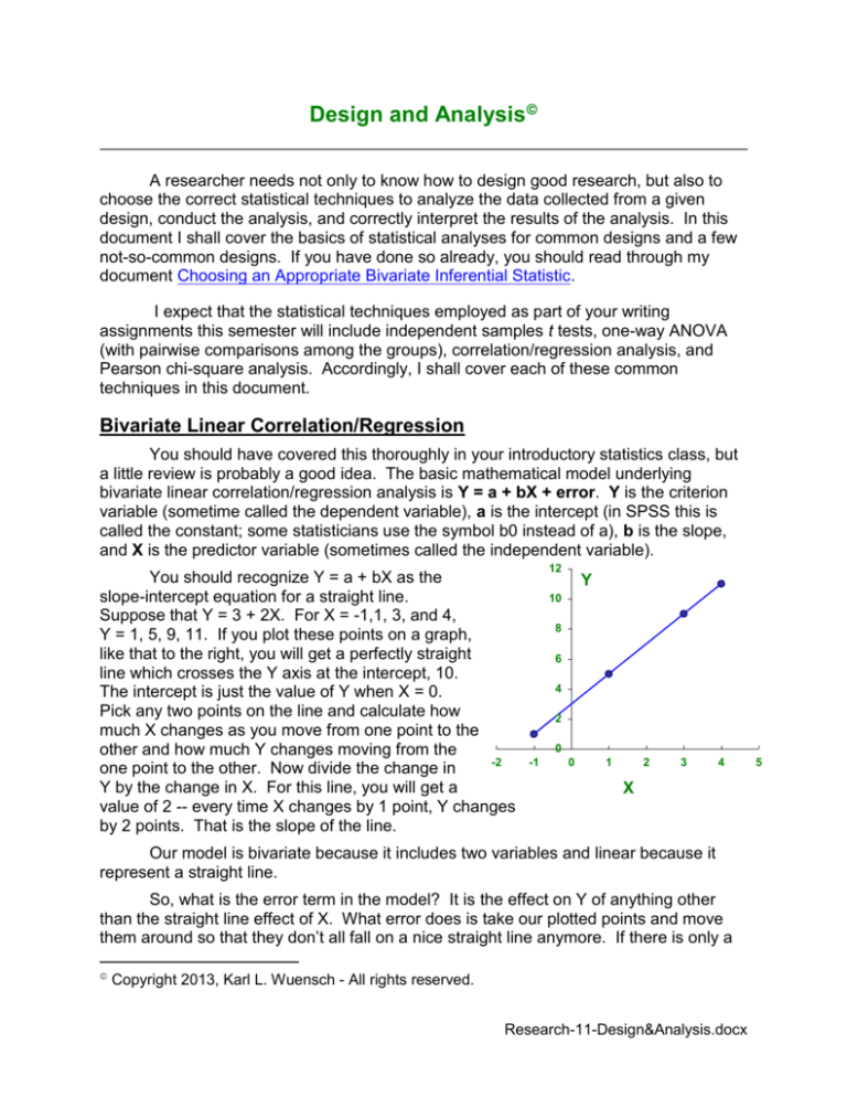
You should recognize Y = a + bX as the
slope-intercept equation for a straight line.
Suppose that Y = 3 + 2X. For X = -1,1, 3, and 4,
Y = 1, 5, 9, 11. If you plot these points on a graph,
like that to the right, you will get a perfectly straight
line which crosses the Y axis at the intercept, 10.
The intercept is just the value of Y when X = 0.
Pick any two points on the line and calculate how
much X changes as you move from one point to the
other and how much Y changes moving from the
-2
one point to the other. Now divide the change in
Y by the change in X. For this line, you will get a
value of 2 -- every time X changes by 1 point, Y changes
by 2 points. That is the slope of the line.
12
Y
10
8
6
4
2
0
-1
0
1
2
3
4
X
Our model is bivariate because it includes two variables and linear because it
represent a straight line.
So, what is the error term in the model? It is the effect on Y of anything other
than the straight line effect of X. What error does is take our plotted points and move
them around so that they don’t all fall on a nice straight line anymore. If there is only a

Copyright 2013, Karl L. Wuensch - All rights reserved.
Research-11-Design&Analysis.docx
5
2
little error, most of the plotted points will be close to the line. If there is a lot of error,
most the plotted points will be far from the line.
In a regression analysis we use our sample data to estimate what the value of
the intercept and the slope in the population. We can then use the resulting
“regression” line to predict values of Y given values of X. A regression analysis also
includes an estimation of the size of the error term, which allows us to estimate how
much we are likely to off when we make a prediction of Y given X.
If we standardize the X and Y variables to mean 0, variance 1 (z scores) and
then compute the regression, the intercept will be 0 and the slope will be a statistic
called the Pearson product moment correlation coefficient, “r” for short. That is, r is the
number of standard deviations that Y increases for each one standard deviation
increase in X. If we square r, we get the coefficient of determination, a statistic that tells
us what proportion of the variance in the Y variable is explained by our model.
If you randomly sampled from a population in which X and Y were not related to
one another, the slope of the regression line computed from the sample data would
almost certainly not be exactly zero, due to random sampling error. Accordingly, it may
be helpful to conduct a test of significance of the null hypothesis that the slope for
predicting Y from X is zero -- that is, there is no change in Y when X changes. This is
equivalent to testing the null hypothesis that the Pearson r between X and Y is zero.
This test statistic most often used here is Student’s t statistic, and it is easily computed
by hand or by SPSS or another statistical package.
You should refresh your understanding of the details of correlation/regression
analysis by reading the following documents:


Bivariate Linear Correlation
Bivariate Linear Regression
If you are not already an expert at using SPSS to conduct correlation/regression
analysis, including multiple regression analysis, you should read and work through my
handout on that topic:

Correlation and Regression Analysis: SPSS
The General Linear Model
In its most general form, the GLM (general linear model) uses linear modeling
techniques to describe the relationship between a set of Y variables and a set of X
variables. That is, a weighted linear combination of Y1, Y2, ....., Yq is correlated with a
weighted linear combination of X1, X2, ......, Xp, where ‘q’ is the number of Y variables
and ‘p’ is the number of X variables. So what is a weighted linear combination? It is a
combination of variables that takes this form: b1X1 + b2X2 + ....... + bpXp. When there
are multiple X variables and multiple Y variables the analysis is called a canonical
correlation/regression. Every other analysis we shall cover here can be considered to
be a special case of the general linear model, generally a special case in which the
model has been simplified somewhat from that which we call a canonical
correlation/regression analysis. For example, the bivariate linear correlation/regression
3
analysis that we just covered is a simplification of the canonical correlation/regression in
that we have only one X variable and only one Y variable.
Dummy Variable Coding
The variables in a linear model must be either continuous or dichotomous, but we
can include categorical variables by representing them with a set of so-called dummy
variables. Suppose we wish to develop a model to predict a person’s political
conservatism from the person’s ethnic identity. For the population with which we are
dealing, imagine that it is appropriate to categorize ethnic identity as having the
following values: African American, European American, Native American, Hispanic,
and Other. One always needs k-1 dummy variables to code k groups, so we shall need
4 dummy variables. The most simple type of dummy variable coding involves assigning
a score of 1 to subjects that are considered to be in a particular group and a score of 0
to those who are not considered to be in that group. For our example here, dummy
variable 1, D1, would indicate whether or not the subject was African American (1 = yes,
0 = no). D2 would indicate whether or not the subject was European American, D3
Native American, and D4 Hispanic. We do not need a dummy variable for the fifth
category, since a subject who gets zeros on D1, D2, D3, and D4 is known to be in the fifth
category. Do note that the categories must be mutually exclusive and exhaustive -- that
is, a subject must belong to one and only one category.
Several Flavors of the GLM











Bivariate Correlation/Regression: One continuous Y, one X, both continuous.
Independent Samples T Test: One continuous Y one dichotomous X,.
Pearson Chi-Square, 2 x 2: One dichotomous Y, one dichotomous X.
Multiple Regression: One continuous Y, two or more continuous X’s.
Polynomial Regression: One continuous Y, one or more continuous X’s and
their powers. This allows the GLM to model data where the regression line is
curved (as in quadratic, cubic, etc.)
One-Way Independent Samples ANOVA: One continuous Y, one dummy
coded categorical X.
Factorial Independent Samples ANOVA: One continuous Y, two or more
dummy coded categorical X’s.
Correlated Samples T and ANOVA: Subjects or blocks represented as an
additional X in a factorial design (the univariate approach) or coded as
differences in multiple Y’s (the multivariate approach).
ANCOV: One continuous Y, one or more dummy coded categorical X’s, one or
more continuous X’s.
MANOVA: Two or more continuous Y’s, one or more dummy coded categorical
X’s.
Discriminant Function Analysis: One or more categorical Y’s, two or more
continuous X’s.
4
Logistic Regression: One categorical Y (usually dichotomous), one or more
continuous X’s and, optionally, one or more dummy-coded categorical X’s.
Canonical Correlation/Regression: Two or more Y’s and two or more X’s.
Independent Samples T Test
Suppose that you wish to determine if there is a relationship between a
dichotomous variable and a normally distributed variable. For example, suppose you
employed a randomized posttest only control group design to determine whether getting
psychotherapy or not (the dichotomous variable) affects a measure of psychological
wellness (the normally distributed variable). In your data file each subject has two
scores. For the X variable, subjects in the control group have a score of 0 and subjects
in the psychotherapy group have a score of 1 (you could use any other two numeric
codes, but 0 and 1 are traditional, because they make the calculations easier, which
was a consideration back in the dark ages when we did not have computing machines).
You use the GLM to predict Y from X. Assuming that you use the 0,1 coding for X, the
intercept is the mean of the control group and the slope is the difference between the
two groups’ means. Student’s t is used to test the null hypothesis that the slope is zero.
If that test is statistically significant, then we reject that null hypothesis and conclude
that the difference in the group means is significant -- that is, that mean psychological
wellness in those who receive psychotherapy differs significantly from that of those who
do not receive psychotherapy. Since we used a well-controlled experimental design,
that means that the psychotherapy caused the difference in wellness. We could still use
the same analysis with data from a nonexperimental design, but could not make strong
causal inferences in that case.
The Pearson r between dichotomous X and normally distributed Y is called a
point-biserial r. We can square it to obtain the proportion of the variance in Y that is
explained by X.
A mathematically equivalent way to calculate the t test is to find the ratio of the
difference between the two means divided by the standard error of the difference
between the two means. This is probably how you learned to do it in your introductory
statistics class.
You should note that the t I have described assumes that Y is normally
distributed and it also assumes homogeneity of variance (equality of the variance of Y in
the two populations). There is another form of this test, called the separate variances t
test (as opposed to pooled variances), which does not assume homogeneity of
variance. I am of the opinion that you should employ the separate variances test
whenever the two samples sizes differ from one another or, even with equal sample
sizes, when the ratio of the larger sample variance to the smaller sample variance
exceeds 4 or 5. Most statistical packages report both the pooled variances t and the
separate variances t, but you have to have the good sense to choose the correct one.
If you do not remember well from your introductory statistics class all the details
of conducting and interpreting independent samples t tests, please read the following
document:

Two Group Parametric Hypothesis Testing
5
If you are not already an expert at using SPSS to conduct correlation/regression
analysis, you should read and work through my handout on that topic:

T Tests and Related Statistics: SPSS
One-Way Independent Samples ANOVA
Remember my example of dummy coding above, where we wanted to develop a
model to predict a person’s political conservatism from the person’s ethnic identity? We
use political conservatism as the Y variable (hopefully it is normally distributed) and our
set of four dummy variables as the X variables. We conduct a multiple regression to
predict Y from a linear combination of the X’s. If you have read and worked your way
through my handout Correlation and Regression Analysis: SPSS, then you already have
had enough of an introduction to multiple regression to understand what I say here
about how it is used to conduct an ANOVA.
The F that tests the null hypothesis that the multiple correlation coefficient, R, is
zero in the population is the omnibus test statistic that we want here. If that null
hypothesis is true, then knowing a person’s ethnic identity tells us nothing about that
person’s political conservatism -- stated differently, mean political conservatism is the
same in all five ethic identity populations. The R2 from this analysis is what is more
commonly called eta-quared, 2, in the context of ANOVA, the proportion of the
variance in Y that is accounted for by X.
A mathematically equivalent way to conduct the ANOVA is to compute F as the
ratio of the among groups variance to the within groups variance. That is probably how
you learned to do ANOVA in your introductory statistics class.
If you do not remember well from your introductory statistics class all the details
of conducting and interpreting one-way independent samples ANOVA, please read the
following document:

One-Way Independent Samples Analysis of Variance
If you have three or more groups in your ANOVA, you probably will want to
conduct multiple comparisons among the means of the groups or subsets of groups.
There is quite a variety of procedures available for doing this. If you have only three
groups, I recommend Fisher’s procedure (more commonly known as the LSD test). If
you have four or more groups, I recommend the REGWQ procedure. If you are not
comparing each mean with each other mean, but rather are making a small number of
planned comparisons, I recommend the Bonferroni or the Sidak procedure. If you do
not remember from your introductory statistics class what these procedures are or why
they are employed (to control familywise error rate), please read the following
document:

One-Way Multiple Comparisons Tests
If you are not already an expert at using SPSS to conduct one-way independent
samples ANOVA with multiple comparisons, you should read and work through my
handout on that topic:

One-Way Independent Samples ANOVA with SPSS
6
Chi-Square Contingency Table Analysis
The Pearson Chi-square is commonly used for two-dimensional contingency
table analysis -- that is, when you seek to investigate the relationship between two
categorical variables. If you did not cover this statistics in your introductory course or if
you need a refresher on this topic, please read the document Common Univariate and
Bivariate Applications of the Chi-square Distribution, especially the material from the
heading “Pearson Chi-Square Test for Contingency Tables” to the end of the document.
To learn how to use SPSS to conduct Pearson Chi-square, read the document TwoDimensional Contingency Table Analysis with SPSS.
An alternative analysis is use of the log-linear model. Using this approach we
construct and evaluate a model for predicting the natural logarithm of cell frequencies
from effects that reflect the marginal distributions of the variables and associations
between and among the variables.
Log-linear models employ Likelihood-Ratio tests of the null hypothesis. The two
likelihoods involved in such a test are:

The likelihood of sampling data just like those we got, assuming that the null
hypothesis (independence of the variables) is true.

The likelihood of sampling data just like those we got, assuming that a particular
alternative hypothesis is true, where that particular alternative hypothesis is the
one which would maximize the likelihood of getting data just like those we got.
To the extent that the latter likelihood is greater than the first likelihood, we have
cast doubt on the null hypothesis.
Contrast this approach with that of traditional hypothesis testing, in which we
assume that the null hypothesis is true and then compute p, the probability of obtaining
results as more discrepant with the null hypothesis than are those we obtained. The
greater that discrepancy (the lower p), the more doubt we have cast on the null
hypothesis.
While the log-linear analysis could be applied to a two-dimensional contingency
table, it is usually reserved for use with multidimensional tables, that is, when we are
investigating the relationships among three or more categorical variables. If you would
like to see how SPSS can be used to analyze multidimensional contingency tables, read
the documents under the heading “Multidimensional Contingency Table Analysis” on my
Statistics Lesson Page.
We have now covered all of the basic analyses that are included in the set of
analyses I expect to be employed in your writing assignments. You should, however,
also be familiar with more complex analyses, both those included in our text book and
others, so I shall continue.
Factorial Independent Samples ANOVA
If you have not already read the document An Introduction to Factorial Analysis
of Variance, please do so now. The factorial ANOVA is also a special case of the GLM,
with the categorical variables and their interaction dummy coded. Consider the case of
7
an A x B, 3 x 3 factorial design. It requires two dummy variables to code factor A (I’ss
call them A1 and A2) and another two dummy variables to code factor B( B1 and B2).
The A x B interaction is represented by four dummy variables, each the product of one
of the A dummy variables and
The following table shows the correspondence between levels of A and B and scores on
the dummy variables.
Level of A
Level of B
A1
A2
B1
B2
A1B1
A1B2
A2B1
A2B2
1
1
1
0
1
0
1
0
0
0
1
2
1
0
0
1
0
1
0
0
1
3
1
0
0
0
0
0
0
0
2
1
0
1
1
0
0
0
1
0
2
2
0
1
0
1
0
0
0
1
3
1
0
0
1
0
0
0
0
0
3
2
0
0
0
1
0
0
0
0
3
3
0
0
0
0
0
0
0
0
The GLM analysis starts by predicting Y from all of the dummy variables, that is,
Y = a + b1A1 + b2 A2 + b3 B1 + b4 B2 + b5 A1B1 + b6A1B2 + b7A2 B1 + b8A2B2. I shall refer
to the R2 for this model as the R2full. To evaluate each effect in the omnibus ANOVA,
we remove from the full model all of the dummy variables representing that effect and
then we test the significance of the resulting decrease in the model R2.
To test the significance of the A x B interaction, we obtain R2 for predicting Y
from A1, A2, B1, and B2 and then subtract the resulting R2 from R2full. That is, we see
how much R2full drops when we remove A1B1, A1B2, A2 B1, and A2B2 from the model. A
partial F test is used to test the null hypothesis that the decrement in R2 is zero, which is
equivalent to the null hypothesis that there is no interaction between factors A and B.
This F is evaluated with 4 df in the numerator – one df for each dummy variable that
was removed from the full model.
The main effect of A is tested by removing A1 and A2 from the full model and
computing a partial F (on 2 df ) to test if the resulting decrement in R2 is significant. The
main effect of B is tested by removing B1 and B2 from the full model and computing a
partial F (on 2 df ) to test if the resulting decrement in R2 is significant.
This sounds pretty tedious, doesn’t it. Fortunately a good statistical package will
take care of all of this for you, from creating the dummy variables to conducting the F
tests.
Again, this is probably not how you learned to conduct factorial ANOVA in your
introductory statistics class. Furthermore, you probably only covered orthogonal
factorial ANOVA (where the cell sizes are all
equal). The analysis is more complex when the
8
cell sizes are not equal. Suppose that we are conducting a two-way ANOVA where the
factors are ethnic group (Caucasian or not) and political affiliation (Democratic or not)
and the criterion variable is a normally distributed measure of political conservatism.
After we gather our data from a random sample of persons from the population of
interest, we note that the cell sizes differ from one another, as shown in the table below:
Political Affiliation
Ethnicity
Democrat
Not Democrat
Caucasian
40
60
Not Caucasian
80
20
The cell sizes are different from one another because the two factors are
correlated with one another -- being Caucasian is significantly negatively correlated with
being a Democrat,  = .41, 2(1, N = 200) = 33.33, p < .001. The correlation between
the two factors results in their being a portion of the variance in the criterion variable
that is ambiguous with respect to whether it is related to ethnicity or to political affiliation.
Look at the Venn Diagram above. The area of each circle represents the variance in
one of the variables. Overlap between circles represents shared variance (covariance,
correlation). The area labeled “a” is that portion of the conservatism (the criterion
variable) that is explained by the ethnicity factor and only the ethnicity factor. The area
labeled “c” is that portion of conservatism that is explained by the political affiliation
factor and only the political affiliation factor. Area “b” is the trouble spot. It is explained
by the factors, but we cannot unambiguously attribute it to the “effect” of ethnicity alone
or political affiliation alone. What do we do with that area of redundancy? The usual
solution is to exclude that area from error variance but not count it in the treatment
effect for either factor. This is the solution you get when you employ Type III sums of
squares in the ANOVA. There are other approaches that you could take. For example,
one could conduct a sequential analysis (using Type I sums of squares) in which you
assign priorities. For this analysis one might argue that differences in ethnicity is more
likely to cause differences in political affiliation than are differences in political affiliation
to cause differences in ethnicity, so it would make sense to assign priority to the
ethnicity factor. With such a sequential analysis, area “b” would be included in the
effect of the ethnicity factor. It is not, however, always obvious which factor really
deserves priority with respect to getting credit for area “b,” so usually we use the Type
III solution I mentioned first.
You can find much more detail about factorial ANOVA in the documents linked
under the heading “Factorial ANOVA, Independent Samples” on my Statistics Lesson
Page.
Please read and work through the document Two-Way Independent Samples
ANOVA with SPSS to learn how to use SPSS to conduct factorial ANOVA.
9
Correlated Samples ANOVA
When you have correlated samples, either because you have a within-subjects
factor because you have blocked subjects on some blocking variable, the GLM can
handle the analysis by treating subjects or the blocking variable as an additional factor
in a factorial analysis. For example, suppose that you had 20 subjects and each subject
was tested once under each of three experimental conditions. The GLM would
represent the effect of the experimental treatment with two dummy variables and the
effect of subjects with 19 dummy variables. Very tedious, but again, a good statistical
package will take care of all this for you. This approach is the so-called “univariate
approach.” A more sophisticated approach is the so-called “multivariate approach,”
which is also based on the GLM. It is a special case of a MANOVA. It too will be
included in a good statistical package.
If you are interested in learning more about correlated samples ANOVA, you
should read the documents linked under the heading “Correlated Samples ANOVA” on
my Statistics Lesson Page and also the document One-Way Within-Subjects ANOVA
with SPSS.
Analysis of Covariance
If we have a normally distributed criterion variable, one or more categorical
predictors (also called factors) and one or more continuous predictors (also called
covariates), the GLM analysis that is usually conducted is called an ANCOV. The
categorical predictor are dummy coded and the continuous predictors are not.
Interactions between factors and covariates are represented as products. For example,
suppose that we have one three-level factor (represented by dummy variables A1 and
A2) and one covariate (X). We start by computing R2 for the full model, which includes
as predictors A1, A2, A1X, and A2X. Since the usual ANCOV assumes that the slope
for predicting Y from X is the same in all k populations, our first step is to test that
assumption. We remove from the full model the terms A1X and A2X and then test the
significance of the decrement in R2. If the R2 does not decline significantly, then we
drop those interaction terms from the model. From the model that includes only A1, A2,
and X, we remove X and determine whether or not the R2 is significantly reduced. This
tests the effect of the covariate. From the model that includes only A1, A2, and X, we
remove A1 and A2 and determine whether or not the R2 is significantly reduced. This
tests the effect of factor A. This approach adjusts each effect for all other effects in the
model – that is, the effect of the covariate is adjusted for the effect of factor A and the
effect of factor A is adjusted for the effect of the covariate. Sometimes we may wish to
do a sequential analysis in which we do not adjust the covariate for the factors but we
do adjust the factors for the covariates.
Again, a good statistical package will take care of all this for you. If you have
done so already, do read my document ANCOV and Matching with Confounded
Variables, which includes an example of a simple ANCOV computed with SPSS. If you
would like more details on ANCOV, you may consult the document Least Squares
Analyses of Variance and Covariance – but that document assumes that you have
access to a particular pair of statistics books and that you have learned how to use the
SAS statistical package.
10
Multivariate Statistics
Time permitting, we shall learn some more about multivariate statistics. You can
find my documents explaining these statistics on my Statistics Lesson Page. Start with
the document An Introduction to Multivariate Statistics.
Distribution-Free Statistics
Most of the statistical tests that we have covered involve the use of t or F as test
statistics. When you use t or F you are making a normality assumption. If your data are
distinctly non-normal, you may try using a nonlinear transformation to bring them close
enough to normal. Alternatively, you can just switch to distribution-free statistics,
statistics that make no normality assumption. You can find documents covering these
types of statistics on my Statistics Lesson Page under the heading “Nonparametric and
Resampling Statistics.”
Statistics for Nonexperimental Designs
If you want to test causal models and want to keep your statistics simple, you
had best stick to experimental designs. When you have nonexperimental data, where
pretreatment nonequivalence of groups and other confounding problems are the norm,
you will need to use more complex statistical analysis in an attempt to correct for the
design deficiencies. For example, Trochim explains how measurement error on a
pretest can corrupt the statistical analysis of data from a nonequivalent groups pretest
posttest design -- ANCOV comparing the groups’ posttest means after adjusting for
pretest scores. He suggests correcting for such bias by adjusting the pretest scores for
measurement error prior to conducting the ANCOV. Each subject’s pretest score is
adjusted in the following way: X adj  M x  r xx ( X  M x ) , X is the pretest score, rxx is the
reliability of the pretest, and Mx is the mean on the pretest for the group in which the
subject is included.
Regression Point Displacement Design. Please read and work through the
document Using SPSS to Analyze Data From a Regression Point Displacement Design
Regression-Discontinuity Design. Please read and work through the
document Using SPSS to Analyze Data From a Regression-Discontinuity Design.
Copyright 2013, Karl L. Wuensch - All rights reserved.

Fair Use of this Document