Complex exponential
A discrete-time signal may be complex-valued. In digital communications complex signals arise naturally. A complex
signal may be represented in two forms:
z (n)  Re  z (n)  j Im z (n)  z (n) e j argz ( n ) ; arg  z (n)  tan 1
Im  z (n)
Re  z (n)
Classification of DT signals
Periodic and aperiodic signals: A signal x(n) is said to be periodic if, for some positive real integer N ,
x ( n)  x ( n  N ) .
Energy signals and power signals: A signal x(n) is said to be an energy signal if its energy is finite.
N
E  lim  x(n) .
N 
2
N
 P  0
If the average power of a signal is finite then the signal is called power signal.
N
1
2
x ( n) .

N  2 N  1
N
P  lim
 E  
Simple manipulation of DT signals
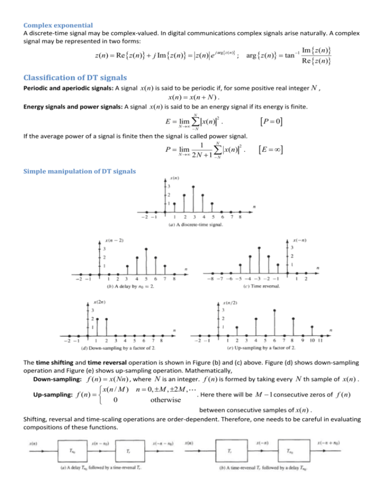
The time shifting and time reversal operation is shown in Figure (b) and (c) above. Figure (d) shows down-sampling
operation and Figure (e) shows up-sampling operation. Mathematically,
Down-sampling: f (n)  x( Nn) , where N is an integer. f ( n) is formed by taking every N th sample of x(n) .
 x(n / M ) n  0,  M , 2M ,
otherwise
 0
Up-sampling: f (n)  
. Here there will be M  1 consecutive zeros of f ( n)
between consecutive samples of x(n) .
Shifting, reversal and time-scaling operations are order-dependent. Therefore, one needs to be careful in evaluating
compositions of these functions.
Analysis of DT systems
T
x(n) 
 y(n)
T  is used to represent a general system. The input signal x(n) is transformed into an output signal y (n) through
the transformation T  .
Classification of systems
1. Linear system:
T
T
 y1 (n) and x2 (n) 
 y2 (n) then for a linear system,
If x1 (n) 
T
a1 x1 (n)  a2 x2 (n) 
 a1 y1 (n)  a2 y2 (n) .
2. Time-invariant system:
T
T
 y (n  n0 ) .
If x(n) 
 y(n) then for a time-invariant system, x(n  n0 ) 
3. BIBO stable system:
A system is BIBO stable if and only if whenever the input signal is bounded as x(n)  A for all n, the output is also
bounded as y(n)  B for all n. If this is violated by the input-output pair the system is not stable.
4. Causal system:
A system is causal if the output y (n) at any time is independent on any value of x ( n  m) for m  0 .
5. Mamoryless system:
A system is said to be memoryless if the output at any time n  n0 depends only on the input at time n  n0 .
6. Invertible system:
A system is said to be invertible if the input to the system may be uniquely determined from the output.
Example
j

n

cos( n) and ii) x(n)  cos(0.125 n) .
17


j N
j n


n  N 
i) x(n  N )  e 16  e 16 cos 

 ; For periodicity, 16 N  2 k1 and 17 N  2 k2 .
 17 17 
k 17
 N  32k1  34k2  1  ; For k1  17 , N  32 17  544
[Ans]
k2 16
A. Determine the periodicity of the signals, i) x(n)  e
16
So, the period of the signal is, 544.
ii)  N  2  
k
 16k . Therefore, N  16.
0.125 
B. Find the even and odd part of the signal x(n)   nu (n) . Hints: xe (n) 
[Ans]
1
 x(n)  x(n) , etc.
2
n
C. Is the system y (n)  x(n) sin
2
linear?
T
T
 y1 (n) and x2 (n) 
 y2 (n) . Then for x(n)  a1 x1 (n)  a2 x2 (n) ,
Let, x1 (n) 
y (n)   a1 x1 (n)  a2 x2 (n)  sin
n
2
 a1 x1 (n) sin
n
2
 a2 x2 (n) sin
n
2
 a1 y1 (n)  a2 y2 (n) .
As the linearity property holds, the system is linear.
D. Is the system y(n)  x(n)  x(n2  n) causal?
For n = -1, y (1)  x(1)  x(2) . As y (n) depends on the future value of x(n) , the system is noncausal.
E. Is the system y(n)  e x ( n ) / x(n  1) stable?
Let x(n)   (n) . Thus, y (n)   . Thus the system is not stable.
F. Is the system y (n)  x(n)  x(n  1) invertible?
Let, x(n)  x1 (n) . Then, y (n)  x1 (n)  x1 (n  1) .
Again let, x(n)  x1 (n)  C . Then, y (n)  x1 (n)  x1 (n  1) .
In both cases the output is the same. Hence, the system is not invertible.
G. Is the system y (n)  2nx(n) time-invariant?
T
 y1 (n) and x1 (n)  x(n  n0 ) . Then, y1 (n)  2nx1 (n)  2nx(n  n0 ) .
Let, x1 (n) 
If the system is time-invariant, y(n  n0 )  2(n  n0 ) x1 (n  n0 ) .
Here, y1 (n)  y (n  n0 ) . Hence the system is time-variant.
[Ans]
Response of LTI systems to arbitrary inputs: The convolution sum
We denote the response of a system to unit sample sequence as impulse response, h(n).
h(n)  T [ (n)]
For a time-invariant system, h(n  k )  T [ (n  k )] .

y (n)  T [ x(n)] =  T [  x(k ) (n  k )] 
Now,
k 

y ( n) 

 x(k )T [ (n  k )]
k 


k 
k 
 x ( k ) h( n  k )  x ( n )  h ( n )  h ( n )  x ( n )   h ( k ) x ( n  k )
The above operation is called convolution operation.
Steps to perform convolution:
1. Change the variable from n to k: x(n), h(n)  x (k ), h(k ) .
2. Perform the folding operation: h(k )  h(k ) .
y (n0 ) 
3. Perform the shifting operation: h(k )  h(n0  k ) .
4. Multiplication: x(k )h(n0  k )  vn0 (k ) .
5. Summation: y(n0 ) 
v
n0

 x ( k ) h( n
k 
0
 k)
(k ) .
Example
1. If x(n)=u(n) and h(n) = 0.8nu(n), y(n)=? .
y ( n) 


k 
n
0.8k u (k )  u (n  k )   0.8k 
k 0
1  0.8n 1
; n0
1  0.8
[Ans]
2. x( n)  {1, 2,3,1} , h( n)  {1, 2,1, 1} , y ( n)  ? .


x(k )  {1, 2,3,1}, h(k )  {1, 2,1, 1} ;


 h(k )  {1,1, 2,1}

Lower limit of y (n) is 0-1=-1 and the upper limit is 3+2=5.
T
1*  1* 
  
2 0
Now, y (1)       1 ;
3 0
  
1 0
T
T
1*   2* 
1*  1* 
  
  
2  1 
2 2

y (0) 
 2  2  4 ; y (1)       1  4  3  8
3  0 
3 1
  
  
1  0 
1 0
T
T
T
1*   1* 
1*   0* 
1*   0* 
  
  
  
2  1 
2   1
2 0


y (2) 
 1  2  6  1  8 ; y (3) 
 3 ; y (4)       2
3  2 
3  1 
 3   1
  
  
  
1  1 
1  2 
1  1 
Similarly, y (5)  1 ; y (6)  0 .
Thus, y (n)  {1, 4,8,8,3, 2, 1}
[Ans]

3. Sketch y (n)  x(2n  3), and y (n)  x(8  3n) for x(n)  (6  n)[u (n)  u (n  6)] .
Properties of convolution
1. Commutative property: x(n)  h(n)  h(n)  x(n)
2. Associative property: {x(n)  h1 (n)}  h2 (n)  x(n) {h1 (n)  h2 (n)}
3. Distributive property: x(n) {h1 (n)}  h2 (n)}  x(n)  h1 (n)  x(n)  h2 (n)
# x(n)   (n)  x(n) and x(n)   (n  k )  x(n  k ) . # if x(n)  N1 , h(n)  N 2 , then, y(n)  N1  N 2  1 .
For causal system and causal input the convolution sum becomes, y (n) 
Some common series
n
n
k 0
k 0
 x ( k ) h( n  k )   h ( k ) x ( n  k ) .
Stability of LTI systems
y ( n) 


h(k ) x(n  k ) ; Let, x(n)  A , then, y (n) 


h(k ) x(n  k ) A
k 
k 

Therefore, the output y(n) is always bounded if

h(k ) is always bounded.
k 
Example: h(n)  a nu (n) . S 


k 

h( k )   a 
k
k 0
1
; a 1.
1 a
The sum is finite for a  1 . Hence, the system is stable.
System described by difference equations
Let, a system has h(n)   nu (n) . Therefore the response of the system would be,
y ( n) 


k 


h( k ) x ( n  k )    k x ( n  k )
 y (n  1)    k x(n  1  k )
k 0
The first equation may be written as, y (n)  x(n) 
k 0


k
x(n  k ) .
k 1
Putting k=p+1, y(n)  x(n) 


p 0
p 0
 p1x(n  p 1)  x(n)    p x(n  p 1)  x(n)   y(n  1)
y (n)  x(n)   y (n  1) .
i.e.,
The above equation is called linear constant coefficient difference equation.
The general form of LCCDE is,
M
N
k 0
k 1
y ( n)   b( k ) x ( n  k )   a ( k ) y ( n  k )
(01)
where, the coefficients a(k) and b(k) are constants that define the system. if, all a(k ) s are not zero the system is
recursive. If a(k)=0 the system is non-recursive.
The integer N is called the order of the difference equation or the order of the system.
Difference equations provide a way for computing the response of a system, y(n) to an arbitrary input x(n). It is
necessary to satisfy a set of initial conditions to solve the above equation. For example, if x(n) begins at n=0, the
solution at time n=0 depends on the values of y (1), y (2), , y ( p ) . When the initial conditions are zero, the
system is said to be in initial rest.
The general solution of an LCCDE system is given as, y (n)  yh (n)  y p ( n)
(02)
The homogeneous solution, yh (n) is the response of the system to the initial conditions assuming that the input
x(n)  0 . The particular solution is the response of the system to the input x(n) , assuming zero initial conditions.
The homogeneous solution may be found by assuming a solution of the form,
yh ( n )  z n
(03)
Substituting in the general equation, z n 
N
 a (k ) z
nk
0
k 1
N
Or,
z n  N [ z N   a (k ) z N  k ]  0 ,  z N  a(1) z N 1  a(2) z N 2 
 a( N )  0
k 1
The polynomial in equation (04) is called the characteristic polynomial. It has N roots.
If all the roots are distinct the homogeneous solution will be of the form,
yh (n)  A1 z1n  A2 z2n 
 AN z Nn
If there are m repeated roots, the solution would be,
yh (n)  ( A11  A12 n 
 A1m n m 1 ) z1n  A2 z2n 
 AN z Nn
If there are two complex roots, z1 , z2  a  jb  re  j , the solution would be,
yh (n)  r n ( B1 cos n  B2 cos n )  A3 z3n 
 AN z Nn
(04)
Example:
1. Find yh (n) for the system, y (n)  y (n  1)  y (n  2) .
The characteristic polynomial, z 2  z  1  0 
n
z
1 5
.
2
n
 1 5 
 1 5 
Hence, yh (n)  A1 

A


 ; n  0
2
 2 


 2 
Let the initial conditions be y (0)  0, y (1)  1 . Applying initial conditions,
 1 5 
 1 5 
A1 

  A2 
  1
 2 
 2 
n
n
1  1  5   1  5  

 yh ( n ) 
 
 
5  2   2  


2. Find yh (n) for the system, y (n)  4 y (n  1)  4 y (n  2)  0
A1  A2  0;
The characteristic polynomial, z 2  4 z  4  0; 
A1   A2 
1
5
[Ans]
z1 , z2  2, 2
 yh (n)  ( A11  A12 n)2n
[Ans]
3. Find yh (n) for the system, y (n)  2 y (n  1)  2 y (n  2)  0
z1 , z2  1  j1  2e j 3 / 4
The characteristic polynomial, z 2  2 z  2  0; 
 yh ( n ) 
 2  [ A cos 34n  A sin 34n ]
n
1
[Ans]
2
--------------------------------------------------------------------------------------------------------------------For the particular solution it is necessary to find the sequence y p (n) that satisfies the difference equation for the
given x(n) . Table below lists particular solutions for some common inputs.
Example:
1. Find the solution of the difference equation,
y (n)  0.25 y (n  2)  x(n)
for x(n)  u ( n) with y (1)  1 and y (2)  0 .
y p (n)  C1 . Substituting this in the difference equation we get,
For x(n)  u ( n) ,
y p (n)  0.25 y p (n  2)  1 ,
C1  0.25C1  1 ;  C1  4 / 3
or,
Now, the characteristic polynomial is, z 2  0.25  0 
 yh (n)  A1 (0.5)  A2 (0.5)
n
(01)
z  0.5
n
The total solution is, y (n)  A1 (0.5) n  A2 (0.5) n  4 / 3;
n0
(02)
The total solution only applies to n  0 , therefore, we have to derive an equivalent set of initial conditions
and y (1) from the system equation (01).
 y (0)  0.25 y(2)  x(0)  0.25  0  1  1

 y (1)  0.25 y (1)  x(1)  0.25 1  1  1.25
Using equation (02), 1  A1  A2  4 / 3; 1.25  0.5 A1  0.5 A2  4 / 3
 y(n)  0.25(0.5)  (1/12)(0.5)  4 / 3; n  0
n
n
 A1  0.25, A2  1/12
[Ans]
y (0)
2. Find the response of the system y (n)  y (n  1)  y (n  2)  0.5 x(n)  0.5 x(n  1) to the input x(n)  0.5n u (n)
with initial condition y (1)  0.75 and y (2)  0.25 .
 z  0.5(1  j 3)  e  j / 3 .
The characteristic equation of the system is, z 2  z  1  0 .
Thus,
yh (n)  A1e j n / 3  A2 e  j n / 3
And,
y p (n)  C1 0.5n u(n); n  0
Substituting this in the difference equation we get, C1 0.5n  C1 0.5n 1  C1 0.5n  2  0.5  0.5n  0.5  0.5n 1
 C1  0.5
 C1  2C1  4C1  0.5  1 ;
Therefore,
y (n)  A1e
j n / 3
 A2e
 j n / 3
 0.5  0.5 ; n  0
n
 y(0)  y(1)  y(2)  0.5 x(0)  0.5 x(1)  A1  A2  0.5  1
Applying initial conditions, 
 1
e j / 3

j / 3
 j / 3
 0.25  1
 y(1)  y(0)  y(1)  0.5 x(1)  0.5 x(0)  A1e  A2e
 1  j / 3

e
3/ 4 

1   A1   0.5 
 A1 
j 2









 j / 3  
e
3  1 j / 3
 A2 
  A2  0.75
 e
 3 / 4
 2

This yields, y (n)  0.5n 1 
3
n
 (n  1)
sin
 3 sin
2
3
3
3. Find unit sample response, h(n) of the system described as y (n) 
[Ans]
3
1
y (n  1)  y (n  2)  x(n)  x(n  1) .
4
8
The impulse response is the response of a system with x(n)   (n) and initial rest conditions.
The characteristic equation is, z 2 
n
3
1
z 0
4
8
1
1
 ( z  )( z  )
2
4
1 1
 z , .
2 4
n
1
1
Hence,
y (n)  A1    A2    0; n  0
2
4
With initial rest condition, y (1)  y (2)  0 , it follows that,
3
1

y
(0)

y
(

1)

y (2)  x(0)  x(1)  1  A1  A2

4
8
 A1  2, A2  3

3
1
3
1
1
1
 y (1)  y (0)  y (1)  x(1)  x(0)   1    A  A
1
2

4
8
4
4 2
4
n
n
n
  1 n
1
1
1 
Hence, h(n)  2    3   ; n  0 , or, h(n)   2    3    u (n)
[Ans]
2
4
 4  
  2 
4. Find the response of the system of problem -3 for the input x(n)  u (n)  u (n  10) with zero initial condition.
Let, s ( n) be the step response of the system. Then, y (n)  s (n)  s (n  10) .
k
k
n
n 
1
1 
s (n)  h(n)  u (n)   h(k )    2    3   
Now,
n0
2
4




k 0
k 0 



n 1
n 1
 1  (1/ 2)
1  (1/ 4) 
n
n
s(n)   2
3
Or,
 u (n)  2(1/ 2)  (1/ 4)  u(n)
1

1/
2
1

1/
4


Thus,
y (n)   2(1/ 2) n  (1/ 4) n  u (n)   2(1/ 2) n 10  (1/ 4) n 10  u ( n  10)
[Ans]
5. Find h(n) of the system described as: y (n)  3 y (n  1)  2 y (n  2)  x(n)  3 x(n  1)  2 x(n  2) .
h(n)  3h(n  1)  2h(n  2)   (n)  3 (n  1)  2 (n  2)


z 2  3z  2  0; 
z1 , z2  1, 2
h(n)  C1  C2  2  u (n)  C3 (n)
n
Now, from the difference equation, h(0)=1; h(1)=3+3=6, h(2)=18-2+2=18
(01)
Putting these in equation (01) we get,
1  C1  C2  C3

 6  C1  2C2
 18  C  4C
1
2

 C1  6, C2  6, C3  1
 h(n)   6  6  2n  u ( n)   ( n)  6  2 n  1 u ( n)   ( n)
[Ans]
6. Determine the response y (n) , n  0 , of the system described by the second –order difference equation
y (n)  3 y (n  1)  4 y (n  2)  x(n)  2 x(n  1) when the input sequence is x(n)  4n u (n) .
Here, Ch. Eq.: z 2  3 z  4  0  ( z  1)( z  4)  0 
Therefore,
z1 , z2  1, 4 .
yh (n)  c1 (1)  c2 (4) .
n
n
As the system root contains one characteristic root, y p (n)  c3n(4)n . Putting this in system equation we get,
c3n(4) n u (n)  3c3 (n  1)(4) n 1 u (n  1)  4c3 (n  2)(4) n  2 u (n  2)  (4) n u (n)  2(4) n 1 u (n  1)
For n  2 none of the unit step terms vanish. We can solve c3 for any n  2 . Use n=2
32c3  12c3  24  c3 
6
.
5
Thus, the total solution of the difference equation is, y (n)  c1 (1) n  c2 (4) n 
Assume that the initial conditions, y (1)  y (2)  0 .
6
n  4n .
5
 y (0)  c1  c2  3 y (1)  4 y ( 2)  1  1
1
26

 c1   , and c2 
Then, 
24
25
25
 y (1)  c1  4c2  5  3 y (0)  4 y ( 1)  6  9
1
26
6
(1) n  (4) n  n(4) n ; n  0
Hence, the zero-state response of the system is, y (n)  
25
25
5
[Ans]
Correlation of D.T. signals
The correlation of two sequences is an operation defined by the relation,
rxy (l ) 
ryx (l ) 


x(k ) y (k  l ) 

 x (k  l ) y (k )
k 
k 


k 
k 
 y (k ) x(k  l )   y (k  l ) x (k )
 rxy (l )  ryx (l )
The computation of correlation sequence involves the same operation as convolution except for the folding
rxy (l )  x(l )  y (l ) .
operation,
If y (n)  x(n) , we have autocorrelation: rxx (l ) 

 x(k ) x(k  l ) .
k 
If x(n) and y (n) are causal sequences of length N, (0  n  N  1) ,then,
N  p 1
rxy (l ) 

x(k ) y (k  l ) , where,
for l  0 , i  l & p  0 and for l  0 , i  0 & p  l .
k i
Applications:
Correlation measures the degree to which two signals are similar. This concept is often used in radar, sonar and
digital communication.
1. Let, x(n) is the transmitted signal. y (n) is the received signal which is the delayed version of the input
signal. Then, y (n)   x(n  l )  w(n) . Correlation of x(n) and y (n) will be maximum at lag l from where
we can measure the distance of a target.
2. In communication system the concept of correlation is used to determine whether the received signal is
zero or one.
To transmit zero we send x0 ( n) , 0  n  L 1 ;
To transmit one we send x1 (n) , 0  n  L 1
Signal received by the receiver is, y(n)  xi (n)  w(n); i  0,1 . The receiver compares y (n) with
x0 (n) and x1 (n) {pattern available in receiver} to determine the signal that better match y (n) .
Example: Determine the correlation between the two sequences x(n) and y (n) given below.
x(n)  {2, 1,3, 7,1, 2, 3, 7,1, 2, 3}

y(n)  {1, 1, 2, 2, 4,1, 2,5}

Properties of correlation sequences
Let, x(n) and y (n) are two finite energy sequences. Now, the energy of the combined sequence, ax(n)  y (n  l ) :
E

 ax(n)  y(n  l )
n 
2
 a 2 rxx (0)  ryy (0)  2arxy (l )  0
 rxx (0) rxy (l )   a 
    0 for any finite value of a .
 rxy (l ) ryy (0)   1 
This equation can be rewritten as:  a 1 
 rxx (0) rxy (l ) 
 is positive semi-definite.
r
(
l
)
r
(0)
xy
yy


Thus, the matrix 
This implies, rxx (0)ryy (0)  rxy2 (l )  0 ,
For, y (n)  x(n) ,
i.e., rxy (l )  rxx (0)ryy (0) 
Ex E y .
rxx (l )  Ex .
Thus autocorrelation attains its maximum value at zero lag.
Quadratic Forms
A quadratic form ‘q’ in ‘n’ variables x1 , x2 ,
x1 x2 , x1 x3 ,
, xn is a linear combination of terms x12 , x22 ,
, xn2 and cross terms
.
If n=3,
 q  a11 x12  a22 x22  a33 x32  a12 x1 x2  a21 x2 x1  a13 x1 x3  a31x3 x1  a23 x2 x3  a32 x3 x2 .
This sum can be written compactly as a matrix product,
q(x)  xT Ax , x  n , A  n  n
When A  AT then, q(x)  0 for all x  0 if and only if A is positive definite (all eigenvalues are positive). In this case
‘q’ is called positive definite.
  x1  x3
 0   x1 x3 
0
I  A  0  

 0; 


 x3   x2
 0    x3 x2 
  2  ( x1  x2 )  ( x1 x2  x32 )  0 ;  would be positive if ( x1 x2  x32 )  0 .
Note that, a in the energy equation is an attenuation factor. Therefore the roots of a must not be complex. This
implies, rxx (0)ryy (0)  rxy2 (l )  0 .
Detection and estimation of periodic signals in noise
The period of a signal is first estimated by autocorrelating the noisy signal. The noisy signal is then cross-correlated
with a periodic impulse train of period equal to that of the signal. The resulting cross-correlation function is the
signal estimate.
N p  Period of x(n), and N  length of signal
s ( n )  x ( n)  q ( n) ;
Let,  ( n  kN p ) be the periodic impulse train used for autocorrelation. Let N  be the number of impulses used for
1 N 1
[ x(n)  q(n)] (n  kN p  j) ; k  0,1, 2,
N n j
1 N 1
rs (0) 
For j=0,
[ x(n)  q(n)] (n  kN p ); k  0,1, 2,
N n j
1
rs (0) 
Or,
x(0)  q(0)  x( N p )  q( N p )  x(2 N p )  q(2 N p )  x( N )  q( N )
N
1
As x(n) is periodic, x(n)  x(n  kN p ) ; Thus, rs (0) 
N x(0)  q(0)  q( N p )  q(2 N p )   q( N ) .
N
correlation.
Or,
rs ( j ) 
1
rs (0)  x(0) 
N
N /Np
 q(kN
k 0
Similarly, for the other values of j, rs ( j )
p
) , The second term is zero.
x( j ) , which is the required signal.