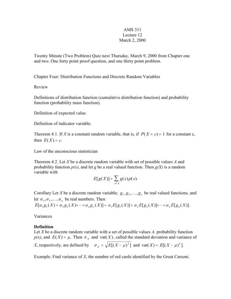
AMS 311
Lecture 12
March 2, 2000
Twenty Minute (Two Problem) Quiz next Thursday, March 9, 2000 from Chapter one
and two. One forty point proof question, and one thirty point problem.
Chapter Four: Distribution Functions and Discrete Random Variables
Review
Definitions of distribution function (cumulative distribution function) and probability
function (probability mass function).
Definition of expected value.
Definition of indicator variable.
Theorem 4.1. If X is a constant random variable, that is, if P( X  c)  1 for a constant c,
then E ( X )  c.
Law of the unconscious statistician
Theorem 4.2. Let X be a discrete random variable with set of possible values A and
probability function p(x), and let g be a real valued function. Then g(X) is a random
variable with
E[ g( X )]   g( x) p( x).
xA
Corollary Let X be a discrete random variable; g1 , g 2 , , g n be real valued functions, and
let  1 ,  2 , ,  n be real numbers. Then
E[ 1 g1 ( X )   2 g 2 ( X )    n g x ( X )]   1 E[ g1 ( X )]   2 E[ g2 ( X )]   n E[ gn ( X )].
Variances
Definition
Let X be a discrete random variable with a set of possible values A, probability function
p(x), and E ( X )   . Then  X and var( X ) , called the standard deviation and variance of
X, respectively, are defined by
X 
E[( X   ) 2 ] and var( X )  E[( X   ) 2 ].
Example: Find variance of X, the number of red cards identified by the Great Carsoni.
Theorem 4.3.
var( X )  E ( X 2 )  [ E ( X )]2 .
Theorem 4.4.
Let X be a discrete random variable with a set of possible values A, and mean . Then
var( X )  0 if an only if X is a constant with probability 1.
Theorem 4.5.
Let X be a discrete random variable; then for constants a and b we have that
var(aX  b)  a 2 var( X ), and  aX  b  | a| X .
Definition
Let X and Y be two random variables and  be a given point. If for all t>0,
P(|Y   |  t )  P(| X   |  t ), then we say that X is more concentrated about  than is Y.
Theorem 4.6. Suppose that X and Y are two random variables with E ( X )  E (Y )   . If
X is more concentrated about  than is Y, then var( X )  var(Y ).