Continuous Random Variables
Discrete random variables assumed values at discrete points. For example, what
values did the poisson random variable assume?
In contrast, continuous random variables take on values along a continuum.
Examples:


T = the time it takes to brush your teeth,
G = the amount of gasoline in your car.
Another example:

L = the length of a baseball game
How is L measured? Do the measurement units determine if L is discrete or continuous?
Associated with a continuous random variable, X, is a probability density function, f(x).
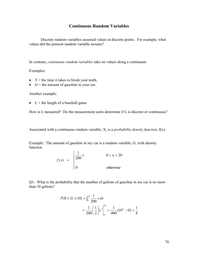
Example: The amount of gasoline in my car is a random variable, G, with density
function
 1
0  x  20
 200 x
f ( x)  

 0
otherwise
Q1: What is the probability that the number of gallons of gasoline in my car is no more
than 10 gallons?
P{0  G  10}  0
10
1
x dx
200
1 1 2

 x
200  2 
10

0
1
1
(10 2  0) 
400
4
70
f(x)
0.1
0.08
0.06
0.04
0.02
0
-2 -1
0
1
2
3
4
5
6
7
8
9
10 11 12 13 14 15 16 17 18 19 20 21 22
Q2: Is the area under the function equal to 1?
P{0  G  20}  0
20
1
x dx
200
1 1 2

 x
200  2 
20

0
1
(20 2  0)  1
400
In fact, to be a legitimate density function, f(x) must satisfy the following conditions:
(1) f(x) > 0 for all x, and
(2)

 f ( x)dx  1
Q3: What is the probability that I have more than 10 gallons in my tank?
P{G > 10} = 1 – P{G < 10} = 1 – ¼ = ¾
71
P{10  G  20}  10
20
Or
1
x dx
200
20
1 1 2
1
3


(20 2  10 2 ) 
 x
200  2  10 400
4
Q4: What is the probability that I have exactly 10 gallons?
P{G  10}  10
10
1
x dx
200
10
1 1 2
1


(10 2  10 2 )  0
 x
200  2  10 400
In fact, for any continuous random variable, X, with density f(x),
P{ X  a}  a f ( x)dx  0
a
An important implication of this for our random variable G is that
P{X < 10}
= P{X = 10} + P{X < 10}
= 0 + P{X < 10},
or
P{X < 10}
= P{X < 10}.
Remember: this is true only for continuous random variables. Now what does this mean?
Recall the notion of relative frequency. If an event E only happens, say, 3 times in an
infinite number of trials, then
nE
3
 lim  0
N  N
N  N
P{E}  lim
An event is said to have probability zero if it can only happen a finite number of times in
an infinite number of trials. You are used to the finite number of occurrences, nE, to be
equal to zero, but in some circumstances, other values are possible!
72
Expectations of Continuous Random Variables
The computation of the expectation (mean or μ) of a continuous random variable
is the continuous analog of the computation for a discrete random variable.
E[ X ]   x p ( x)
for a discrete random variable,
  x f ( x) dx
for a continuous random variable.
Q5: In the gasoline example, do you think that the average amount of gasoline kept in
the tank is less than 10, equal to 10, or more than 10?
To compute E[G]:
E[G ]  0 x f ( x) dx
20
20  1

 0 x 
x dx
 200 
1 20 2

 x dx
200 0
20
 1  1  3

  x
 200  3  0
1
40
1

(20 3  0 3 ) 
 13
600
3
3
The computation of the variance, Var(X) = σ2, of a continuous random variable is the
continuous analog of the computation for a discrete random variable.
Var ( X )   ( x   ) 2 p( x)
  ( x   ) 2 f ( x) dx
for a discrete random variable
for a continuous random variable.
73
Note that it is frequently easier to compute
Var ( X )  E[ X 2 ]   2
  x 2 f ( x) dx   2
In the gasoline example:
 1 
 40 
  0 x 
x  dx   
 200 
 3 
2
20
1 20 3
 40 

x dx   

0
200
 3 
 1  1  4

  x
 200  4 
20
0
 40 
 200   
 3 
Thus
2
2
2
 40 
  
 3 
2

2
200
 22.2
9
   2  22.2  4.71 .
74
Continuous Uniform Random Variables
Suppose the random variable X assumes values between a and b with each value
being equally likely to occur. What should the density function look like?
a
Then
 1
b  a

f ( x)  
0


b
axb
otherwise
Let X be the time until the arrival of the next bus. If X is uniform on [2, 7], what does
f(x) look like?
What is the probability of having to wait more than 5 minutes on the next bus?
P{ X  5}  5
7
Using calculus:
1
dx
5
7
1
1
2
 x  (7  5) 
5 5 5
5
75
Geometrically:
f(x) = 1/5
1/5
2
5
7
To compute the mean of X:
1
5
  E[ X ]  2 x  dx
7
7
 1  1 
    x 2
 5  2  2
1
 (7 2  2 2 )  4.5
10
In general, for a random variable uniform on [a, b]: E[ X ] 
ab
2
(b  a) 2
And the variance is given by: Var ( X ) 
12
(7  2) 2 25

In our example, Var ( X ) 
.
12
12
76
Homework for Continuous Random Variables
(#1) Suppose the random variable X is distributed as
2  2 x

f ( x)  
0

0  x 1
otherwise
(a) Graph f(x).
(b) Prove that f(x) is a real density function.
(c) P{X > ½} =
(d) P{X = ¼} =
(e) P{X > -1} =
(f) P{ ¼ < X < ¾ } =
(g) E[X] =
(h) Var(X) =
(#2) Assume X is uniform on [1, 8].
(a) P{X > 4} =
(b) P{X = 4} =
(c) E[X] =
(d) Var(X) =
77