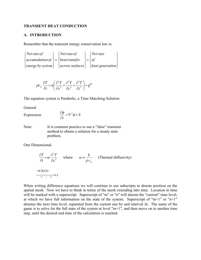
TRANSIENT HEAT CONDUCTION
A. INTRODUCTION
Remember that the transient energy conservation law is:
 Net rate of
  Net rate of
  Net rate


 
 

accumulation of   heat transfer   of

energy by system across surfaces  heat generation 

 
 

c p
  2T  2T  2T 
T
   2  2  2   q 
t
y
z 
 x
The equation system is Parabolic, a Time Marching Solution
General

  2  S
t
Expression
Note:
It is common practice to use a “false” transient
method to obtain a solution for a steady state
problem.
One Dimensional
T
 2T
 2
t
x
where

k
 cp
(Thermal diffusivity)
| x |
i
  x
1 i i1
When writing difference equations we will continue to use subscripts to denote position on the
spatial mesh. Now we have to think in terms of the mesh extending into time. Location in time
will be marked with a superscript. Superscript of "m" or "n" will denote the "current" time level,
at which we have full information on the state of the system. Superscript of "m+1" or "n+1"
denotes the next time level, separated from the current one by and interval t. The name of the
game is to solve for the full state of the system at level "m+1", and then move on to another time
step, until the desired end time of the calculation is reached.
1D conduction difference equation at an Interior node:
Ti m1  Ti m

Ti1  2Ti  Ti1 

t
x 2
Where T is an abbreviation to hide the fact that we haven't decided on a time level for these
terms. This is defined more directly in terms of a time weighting factor "f" as:
Ti  f Ti m 1  (1- f) Ti m
So the longer definition of the difference equation

 
 
Ti m1  Ti m 
m
m
 2 f Ti m11  (1  f ) Ti 1  2 f Ti m1  (1  f )Ti m  f Ti m11  (1  f )Ti 1
t
x

Three specific values of f provide the three main forms of transient time level methods.
f=0
Forward Difference (Explicit Method)
f = 0.5
Crank-Nicolson
f=1
Backward Difference (Implicit Method)
B. FORWARD DIFFERENCE METHOD
a) Introduction
T
m
Taylor series approximation of t o
TO
m 1
 TO
m
m 1
T
 t
t
m
O
t 2  2T

2 t 2
m
O

T TO  To
t  2T 


O mt    ( m  1) t
t
t
2
t 2


m
error
Using our compass notation for spatial grid points, the explicit finite difference equation is:
m 1
m
m
m
m
m
m
m
TE  TW  2TO 
1  TO  TO   TN  TS  2TO




 
t
y 2
x 2
 

+
q 
k
Rearrange
TO
m 1
T m  T m 
 T m  TW m 
q 
 t  N 2 S   t  E
+
  t
2
k
 y

 x


 1
1  m
1  2t  2  2   TO
y  
 x

Assume a uniform grid and let x  y  
For no heat generation:
T
  2T
t
Write the collection of all difference equations as a linear system (E is a matrix).
Tm+1 = E Tm + b
A 
Let
T1m 1
m 1
2
m 1
3
m 1
4
m 1
5
m 1
6
T
T
T

 t
2
(1  4 A)
A
A
(1  4 A)
O
A
A
O
O
A
A
O
(1  4 A)
O
O
(1  4 A)
O
T1m
200 A
A
O
T
100 A
O
A
A
O
m
2
m
m3
m
4
m
5
m
6
T
T
100 A
100 A
O

T
O
A
O
A
(1  4 A)
A
T
0
T
O
O
A
O
A
(1  4 A)
T
0
Example
T3m+1 = A T2 + (1-4A) T3m + A T6m + 100A
b) Truncation error
T
m
 finite difference equation – differential equation

m
1
1  T1m 1 T1m   T0m 2T1m  T2m   1 T  2T 
 
 2


  t  
2
  t x  1
T
m
Expansions
T1m1  T1m  t
T
t
T0  T1  
T
x
T2  T1  
T
x
m
m
m
m
m
1
m
1
m
1

t 2  2T
2 t 2

2  2T
2 x 2

2  2T
2 x 2
m
1

1  T

  t
m
1

t  2T
2 t 2
 1 T

 t

t  2T
2 t 2
m
1

m
1

m
1
3  3T
3! x 3

3  3T
3! x 3
m
1
m
1
m
1

t 4  4T
4! t 4
m
1


m
1

m

m
1

1
 2T
x 2
t 3  3T
6 t 3

m
Substitute into expression for T
T
t 3  3T
3! t 3
m
1
t 3  3T
3! t 3
m
1
m
1
   2T
    2
  x
m
1

22  4T
4! x 4
m
1

 




 
2  4T
12 x 4
m
1

4  6T
360 t 6
m
1

The forward difference method is first order accurate in time and second order in space.
Consistency
A difference method is said to be "consistent" or "compatible" with a differential equation if
the truncation error approaches zero as the size of the increments of the independent
variables approach 0. We are in luck here. Later I will show you examples where this
situation does not hold.
Limit
T
m
0
 0 
 any order
t  0