The Downhill Simplex method
The Downhill Simplex method is a multidimensional optimization method which uses geometric
relationships to aid in finding function minimums. One distinct advantage of this method is that
it does not require taking the derivative of the function being evaluated. Instead it creates its own
pseudo-derivative by evaluating enough points to define a derivative for each independent
variable of the function.
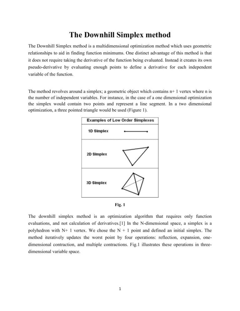
The method revolves around a simplex; a geometric object which contains n+ 1 vertex where n is
the number of independent variables. For instance, in the case of a one dimensional optimization
the simplex would contain two points and represent a line segment. In a two dimensional
optimization, a three pointed triangle would be used (Figure 1).
Fig. 1
The downhill simplex method is an optimization algorithm that requires only function
evaluations, and not calculation of derivatives.[1] In the N-dimensional space, a simplex is a
polyhedron with N+ 1 vertex. We chose the N + 1 point and defined an initial simplex. The
method iteratively updates the worst point by four operations: reflection, expansion, onedimensional contraction, and multiple contractions. Fig.1 illustrates these operations in threedimensional variable space.
1
Reflection involves moving the worst point (vertices) of the simplex (where the value of
the objective function is the highest) to a point reflected through the remaining N points. If
this point is better than the best point, then the method attempts to expand the simplex
along this line. This operation is called expansion.
On the other hand, if the new point is not much better than the previous point, then the
simplex is contracted along one dimension from the highest point. This procedure is called
contraction. Moreover, if the new point is worse than the previous points, the simplex is
contracted along all dimensions toward the best point and steps down the valley. By
repeating this series of operations, the method finds the optimal solution.
2
2.2 Algorithm
The downhill simplex method repeats a series of the following steps:
1. Order and re-label the N+1 points so that f(xN+1) > ... > f(x2) > f(x1)
2. Generate a trial point xr by reflection, such that xr = xg + * (xg  xN+1), where xg is
the centroid of the N best points in the vertices of the simplex
3. If f(x1) < f(xr) < f(xN), replace xN+1 by xr
4. If f(xr) < f(x1), generate a new point xe by expansion, such that xe = xr + * (xr  xg)
5. If f(xe) < f(xr), replace xN+1 by xe, otherwise replace xN+1 by xr
6. If f(xr) > f(xN), generate a new point xc by contraction, such that xc = xg + * (xN+1 
xg).
7. If f(xc) < f(xN+1), replace xN+1 by xc
8. If f(xc) > f(xN+1), contract along all dimensions toward x1. Evaluate the objective
function values at the N new vertices, xi = x1 + * (xi  x1)
It has been reported that efficient values of , , , and  are  = 1.0,  = 1.0,  = 0.5,
and  = 0.5. In this report, we use these parameter settings.
3 Numerical Experiments
3.1 Test Function and Experimental Setup
To verify the performance of the downhill simplex method, we applied the method to a
mathematical test function for continuous optimization problems - the Rosenbrock
function:
(1)
The Rosenbrock function is known as the Banana function. The global optimum is inside
a long, narrow, parabolic shaped flat valley. To find the valley is trivial: however,
3
convergence to the global optimum is difficult and hence this problem has been repeatedly
used to assess the performance of optimization algorithms.[2]
In this report, the dimension of the function is two. The initial vertices of the simplex are
randomly generated in the feasible region.
3.2 Experimental Results
Fig.2(a) shows the history of the design variables of the best vertices. The downhill
simplex method reaches the optimum along the valley. Moreover, the initial simplex is
plotted in Fig.2(b) , and the summary of results of 10 trials are listed in Table 1 .
Fig.2: History of the design variables
Table 1: Experimental results (in 10 trials)
Number of evaluations
Average
234
Standard deviation
53.6
Number of trials when the optimum is found
4
10
The downhill simplex algorithm has a vivid geometrical natural interpretation. A simplex is a
geometrical polytypic which has n + 1 vertexes in a n-dimensional space, e.g. a line segment in
1-dimensional space, a triangle in a plane, a tetrahedron in a 3-dimensional space and so on. In
most cases, the dimension of the space represents the number of independent parameters that
need to be optimized in order to minimize the value of a function: f(takes a vector of n
parameters), where n is the dimension of the space.
To carry out the algorithm, firstly, a set of n+ 1 point is picked in the n-dimensional space, so
that an initial simplex could be constructed. Clearly, the simplex is a n by n+1 matrix, each
column is a point (in fact, a vector of size n) in the n-dimensional space. The simplex consists of
n+1 such vectors. The initial simplex is constructed to be non-degenerate.
Secondly, the target function f is evaluated for all the n+1 vertexes on the simplex. So we can
sort the results and have f(X_1) < f(X_2) . . . < f(X_n) < f( X_{n+1}) . Notice that each X_k is a
vector of size n. Because our goal is to minimize the f, so we define the worst point as
Xw=X_{n+1} and the best point is X_1.
Thirdly, the algorithm iteratively updates the worst point Xw by four possible actions: 1)
reflection, 2) expansion, 3) 1-dimensional contraction, 4) multiple contractions. The following
5
Fig. 1 sketches the actions in a 3-D space with a tetrahedron as the
simplex.
1) Reflection: reflects away Xw through the centroid Xg of the other n best points, to get a
reflected point X_r.
2) Expansion: if the newly found reflected point is better than the existing best point X_1, then
the simplex expands toward the newly found reflected point X_r.
3) Contraction: if the reflected point X_r is no better than the existing best point, then the
simplex contracts along 1-D through the direction of Xw and Xg, from the worst point Xw.
6
4) Multiple contraction: if the newly found X_r is even worst than the existing worst point Xw,
then the simplex contracts along all dimensions toward the existing best point X_1.
The optimal solution of X_1 could be found by iterating the above actions on the updated
condition of the simplex at each step.
7