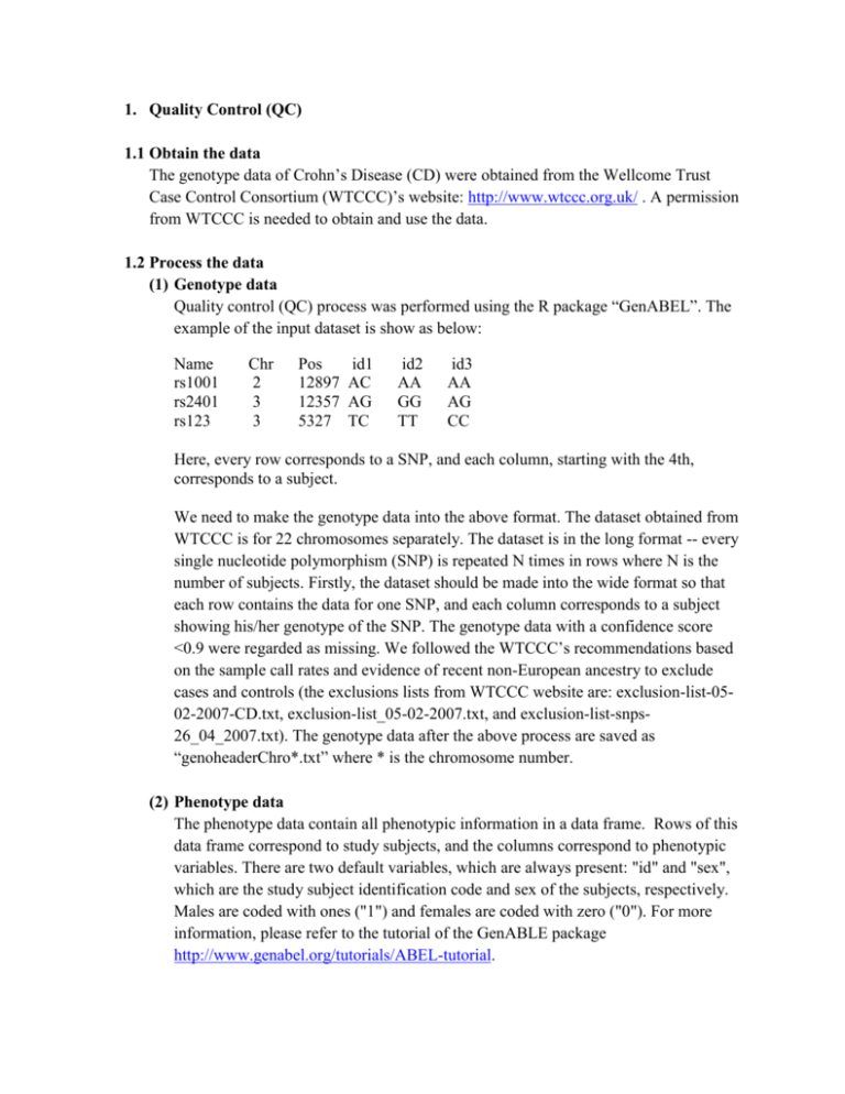
1. Quality Control (QC)
1.1 Obtain the data
The genotype data of Crohn’s Disease (CD) were obtained from the Wellcome Trust
Case Control Consortium (WTCCC)’s website: http://www.wtccc.org.uk/ . A permission
from WTCCC is needed to obtain and use the data.
1.2 Process the data
(1) Genotype data
Quality control (QC) process was performed using the R package “GenABEL”. The
example of the input dataset is show as below:
Name
rs1001
rs2401
rs123
Chr
2
3
3
Pos
12897
12357
5327
id1
AC
AG
TC
id2
AA
GG
TT
id3
AA
AG
CC
Here, every row corresponds to a SNP, and each column, starting with the 4th,
corresponds to a subject.
We need to make the genotype data into the above format. The dataset obtained from
WTCCC is for 22 chromosomes separately. The dataset is in the long format -- every
single nucleotide polymorphism (SNP) is repeated N times in rows where N is the
number of subjects. Firstly, the dataset should be made into the wide format so that
each row contains the data for one SNP, and each column corresponds to a subject
showing his/her genotype of the SNP. The genotype data with a confidence score
<0.9 were regarded as missing. We followed the WTCCC’s recommendations based
on the sample call rates and evidence of recent non-European ancestry to exclude
cases and controls (the exclusions lists from WTCCC website are: exclusion-list-0502-2007-CD.txt, exclusion-list_05-02-2007.txt, and exclusion-list-snps26_04_2007.txt). The genotype data after the above process are saved as
“genoheaderChro*.txt” where * is the chromosome number.
(2) Phenotype data
The phenotype data contain all phenotypic information in a data frame. Rows of this
data frame correspond to study subjects, and the columns correspond to phenotypic
variables. There are two default variables, which are always present: "id" and "sex",
which are the study subject identification code and sex of the subjects, respectively.
Males are coded with ones ("1") and females are coded with zero ("0"). For more
information, please refer to the tutorial of the GenABLE package
http://www.genabel.org/tutorials/ABEL-tutorial.
1.3 Filters used in QC
 SNPs with SNP call rates less than 95% were removed.
 We also removed SNPs based on their minor allele frequencies: the default
minor allele frequency cutoff in the GenABEL R package was used (2.5/N
where N is the number of subjects)
 We used a cutoff of 0.2 for the Hardy-Weinberg Equilibrium (HWE) test’s
false discovery rates, based on combined cases and controls.
Please refer to the example code “QC and LD example.R” for the QC steps.
2. Linkage Disequilibrium
To reduce redundancy of logic trees that genotype indicators of SNPs within a gene can
form, we removed SNPs within each gene sequentially, such that no pair of remaining
SNPs within a gene had linkage disequilibrium (r2≥0.8).
SNP-gene mapping files were obtained from the OpenBioinformatics website
(http://www.openbioinformatics.org/gengen/tutorial_calculate_gsea.html#_Toc21088741
4).
Please refer to the example code “QC and LD example.R” for the LD procedure.
3. Logic regression
We do the analysis using the subjects and SNPs that have passed the above QC and LD
process. The R code “logic regression example.R” is provided in our website
http://www.ualberta.ca/~yyasui/homepage.html, with an example of gene “AARS2” for
495 controls and 251 cases.
The genotype data after QC and LD were made into binary predictors, i.e., indicators of
the minor-allele homozygous and indicators of the heterozygous and the minor-allele
homozygous. Please refer to our example dataset “binary.txt”.
Logic regression is used to model the outcome (e.g., the disease status in a case-control
study) with intersections and/or unions of these binary predictors. To correct for the
inherent instability of the performance measure when searching a large space, we refit the
logic regression 20 times, starting the algorithm with 20 different initial values: this
process was applied to the original dataset as well as 20 datasets obtained by
permutations of the case- control labels. Of the 20 results produced by the 20 starting
values, we selected the best fit, measured by deviance. The result for one gene is a vector
of length 21 (refer to the vector “Dev_per” in the R code), with the first element being the
best fit for the original case-control labels, and the remaining 20 elopements are the best
fit for the 20 permuted case-control labels, respectively.
4. P-value
In Step 3 above, we calculated the 21 (the original + the 20 permuted) best fit dev for one
gene. We do this for all the genes in the study, and the results are then saved in a data
frame with 21 rows and m columns, where m is the number is genes in the study. Please
refer to our example “DevAll.txt” for results of dev.
The P-value for each gene is calculated as the proportion of all permuted BF values of all
genes larger than the gene’s observed BF. This p-value calculation properly takes the
multiple testing into account. Please see our example code for p-value calculation “pvaue calculation.R”.