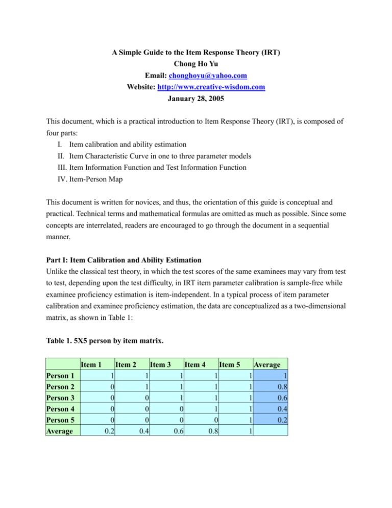
A Simple Guide to the Item Response Theory (IRT)
Chong Ho Yu
Email: chonghoyu@yahoo.com
Website: http://www.creative-wisdom.com
January 28, 2005
This document, which is a practical introduction to Item Response Theory (IRT), is composed of
four parts:
I. Item calibration and ability estimation
II. Item Characteristic Curve in one to three parameter models
III. Item Information Function and Test Information Function
IV. Item-Person Map
This document is written for novices, and thus, the orientation of this guide is conceptual and
practical. Technical terms and mathematical formulas are omitted as much as possible. Since some
concepts are interrelated, readers are encouraged to go through the document in a sequential
manner.
Part I: Item Calibration and Ability Estimation
Unlike the classical test theory, in which the test scores of the same examinees may vary from test
to test, depending upon the test difficulty, in IRT item parameter calibration is sample-free while
examinee proficiency estimation is item-independent. In a typical process of item parameter
calibration and examinee proficiency estimation, the data are conceptualized as a two-dimensional
matrix, as shown in Table 1:
Table 1. 5X5 person by item matrix.
Item 1
Person 1
Person 2
Person 3
Person 4
Person 5
Average
Item 2
1
0
0
0
0
0.2
Item 3
1
1
0
0
0
0.4
Item 4
1
1
1
0
0
0.6
Item 5
1
1
1
1
0
0.8
Average
1
1
1
1
1
1
1
0.8
0.6
0.4
0.2
A simple guide to IRT
2
In this example, Person 1, who answered all five items correctly, is tentatively considered as
possessing 100% proficiency. Person 2 has 80% proficiency, Person 3 has 60%, etc. These scores
in terms of percentage are considered tentative because first, in IRT there is another set of
terminology and scaling scheme for proficiency, and second, we cannot judge a person’s ability
just based on the number of correct items he obtained. Rather, the item attribute should also be
taken into account. In this highly simplified example, no examinees have the same raw scores. But
what would happen if there is an examinee, say Person 6, whose raw score is the same as that of
Person 4 (see Table 2)?
Table 2. Two persons share the same raw scores.
0
0
1
Person 4
Person 5
Person 6
0
0
1
0
0
0
1
0
0
1
1
0
0.4
0.2
0.4
We cannot draw a firm conclusion that they have the same level of proficiency because Person 4
answered two easy items correctly, whereas Person 6 scored two hard questions instead.
Nonetheless, for the simplicity of illustration, we will stay with the five-person example. This nice
and clean five-person example shows an ideal case, in which proficient examinees score all items,
less competent ones score the easier items and fail the hard ones, and poor students fail all. This
ideal case is known as the Guttman pattern and rarely happens in reality. If this happens, the
result would be considered an overfit. In non-technical words, the result is just “too good to be
true.”
Table 1 5X5 person by item matrix (with highlighted average)
Item 1
Person 1
Person 2
Person 3
Person 4
Person 5
Average
Item 2
1
0
0
0
0
0.2
Item 3
1
1
0
0
0
0.4
Item 4
1
1
1
0
0
0.6
Item 5
1
1
1
1
0
0.8
Average
1
1
1
1
1
1
1
0.8
0.6
0.4
0.2
We can also make a tentative assessment of the item attribute based on this ideal-case matrix.
Let’s look at Table 1 again. Item 1 seems to be the most difficult because only one person out of
A simple guide to IRT
3
five could answer it correctly. Again, it is tentatively asserted that the difficulty level in terms of
the passrate for Item 1 is 20%, Item 2 is 40%, etc. This matrix is nice and clean; however, as you
might expect, the issue will be very complicated when some items have the same pass rate but are
passed by examinees of different levels of proficiency.
Table 3. Two items share the same pass rate
Item 1
Person 1
Person 2
Person 3
Person 4
Person 5
Average
Item 2
1
0
0
0
0
0.2
Item 3
1
1
0
0
0
0.4
Item 4
1
1
1
0
0
0.6
Item 5
1
1
1
1
0
0.8
Item 6
1
1
1
1
1
1
Average
0 0.833333
0 0.666667
0
0.5
0 0.333333
1 0.333333
0.2
In the preceding example (Table 3), Item 1 and Item 6 have the same pass rate (20%) and thus they
seem to have the same difficulty level. However, Item 1 was answered correctly by a person who
has high proficiency (83%) whereas Item 6 was not (the person who answered it has 33%
proficiency). It is possible that the text in Item 6 tends to confuse good students. Therefore, the
item attribute of Item 6 is not clear-cut. For convenience of illustration, we call the portion of
correct answers for each person “tentative proficiency” and the pass rate for each item “tentative
item difficulty.” Please do not confuse these “tentative” numbers with the item difficulty parameter
and the person theta in IRT. We will discuss them later.
In short, both the item attribute and the examinee proficiency should be taken into consideration in
order to conduct item calibration and proficiency estimation. This is an iterative process in the
sense that tentative proficiency and difficulty derived from the data are used to fit the model, and
then the model is employed to predict the data. Needless to say, there will be some discrepancy
between the model and the data in the initial steps. It takes many cycles to reach convergence.
Given the preceding tentative information, we can predict the probability of answering a particular
item correctly given the proficiency level of an examinee by the following equation:
Probability = 1/(1+exp(-(proficiency – difficulty)))
Exp is the Exponential Function. In Excel the function is written as exp(). For example:
A simple guide to IRT
4
e0 = 1
e1 = 2.7182= exp(1)
e2 = 7.3890= exp(2)
e3 = 20.0855= exp(3)
Now let’s go back to the example depicted in Table 1. By applying the above equation, we can give
a probabilistic estimation about how likely a particular person is to answer a specific item
correctly:
Table 4a. Person 1 is “better” than Item 1
Person 1
Person 2
Person 3
Person 4
Person 5
Tentative
Difficulty
Tentative
Item 1
Item 2
Item 3
Item 4
Item 5
Proficiency
0.689974 0.645656 0.598688 0.549834
0.5
1
0.645656 0.598688 0.549834
0.5 0.450166
0.8
0.598688 0.549834
0.5 0.450166 0.401312
0.6
0.549834
0.5 0.450166 0.401312 0.354344
0.4
0.5 0.450166 0.401312 0.354344 0.310026
0.2
0.2
0.4
0.6
0.8
1
For example, the probability that Person 1 can answer Item 1 correctly is 0.6899. There is no
surprise. Person 1 has a tentative proficiency of 1 while the tentative difficulty of Item 1 is 0.2. In
other words, he has more than a 50 percent chance to score the item. Person 1 is definitely
“smarter” or “better” than Item 1.
Table 4b. The person “matches” the item.
Person 1
Person 2
Person 3
Person 4
Person 5
Tentative
Difficulty
Tentative
Item 1
Item 2
Item 3
Item 4
Item 5
Proficiency
0.689974 0.645656 0.598688 0.549834
0.5
1
0.645656 0.598688 0.549834
0.5 0.450166
0.8
0.598688 0.549834
0.5 0.450166 0.401312
0.6
0.549834
0.5 0.450166 0.401312 0.354344
0.4
0.5 0.450166 0.401312 0.354344 0.310026
0.2
0.2
0.4
0.6
0.8
1
A simple guide to IRT
5
The probability that Person 5 can answer Item 1 correctly is 0.5. The tentative item difficulty is .2,
and the tentative proficiency is also .2. In other words, the person’s ability “matches” the item
difficulty. When you move your eyes across the diagonal from lower left to upper right, you will
see a “match” (.5) between a person and an item several times. However, when we put Table 1 and
Table 4b together, we will find something strange.
Table 1 5X5 person by item matrix
Item 1
Person 1
Person 2
Person 3
Person 4
Person 5
Average
Item 2
1
0
0
0
0
0.2
Item 3
1
1
0
0
0
0.4
Item 4
1
1
1
0
0
0.6
Item 5
1
1
1
1
0
0.8
Average
1
1
1
1
1
1
1
0.8
0.6
0.4
0.2
According to Table 4b, the probability of Person 5 answering Item 5 correctly is .31, while that of
answering Item 1 correctly is .5. But actually, Person 5 got no points in Item 1 whereas he obtained
one point in Item 5! As mentioned before, the data and the model do not necessarily fit together.
This residual information can help a computer program, such as Bilog, to further calibrate the
estimation until the data and the model converge. Figure 1 is an example of Bilog’s calibration
output, which shows that it takes ten cycles to reach convergence.
Figure 1. Bilog’s Phase 2 partial output
CALIBRATION PARAMETERS
MAXIMUM NUMBER OF EM CYCLES:
MAXIMUM NUMBER OF NEWTON CYCLES:
CONVERGENCE CRITERION:
ACCELERATION CONSTANT:
10
2
0.0100
1.0000
A simple guide to IRT
6
Part II: Item Characteristic Curve (ICC)
After the item parameters are estimated, this information can be utilized to model the response
pattern of a particular item by using the following equation:
P = 1/(1+exp(-(theta – difficulty)))
From this point on, we give proficiency a special name: Theta, which is usually denoted by the
Greek symbol . After the probabilities of giving the correct answer across different levels of  are
obtained, the relationship between the probabilities and  can be presented as an Item
Characteristic Curve (ICC), as shown in Figure 2.
Figure 2. Item Characteristic Curve
In Figure 2, the x-axis is the theoretical theta (proficiency) level, ranging from -5 to +5. Please
keep in mind that this graph represents theoretical modeling rather than empirical data. To be
specific, there may not be examinees who can reach a proficiency level of +5 or fail so miserably
as to be in the -5 group. Nonetheless, to study the “performance” of an item, we are interested in
knowing, given a person whose  is +5, what the probability of giving the right answer is. Figure 2
shows a near-ideal case. The ICC indicates that when  is zero, which is average, the probability of
answering the item correctly is almost .5. When  is -5, the probability is almost zero. When  is
+5, the probability increases to .99.
A simple guide to IRT
7
IRT modeling can be as simple as using one parameter or as complicated as using three parameters,
namely, A, B, and G parameters. Needless to say, the preceding example is a near-ideal case using
only the B (item difficulty) parameter, keeping the A parameter constant and ignoring the G
parameter. These three parameters are briefly explained as follows:
1. B parameter: It is also known as the difficulty parameter or the threshold parameter. This
value tells us how easy or how difficult an item is. It is used in the one-parameter (1P) IRT model.
Figure 3 shows a typical example of a 1P model, in which the ICCs of many items are shown in one
plot. One obvious characteristic of this plot is that no two ICCs cross over each other.
Figure 3. 1P ICCs.
2. A parameter: It is also called the discrimination parameter. This value tells us how effectively
this item can discriminate between highly proficient students and less-proficient students. The
two-parameter (2P) IRT model uses both A and B parameters. Figure 4 shows a typical example of
a 2P model. As you can notice, this plot is not as nice and clean as the 1P ICC plot, which is
manifested by the characteristic that some ICCs cross over each other.
A simple guide to IRT
8
Figure 4a. 2P ICC
Take Figure 4b (next page) as an example. The red ICC does not have a high discrimination. The
probability that examinees whose  is +5 can score the item is 0.82, whereas the probability that
examinees whose  is -5 can score it is 0.48. The difference is just 0.82 - 0.48 = 0.26. On the other
hand, the green ICC demonstrates a much better discrimination. In this case, the probability of
obtaining the right answer given the  of +5 is 1 whereas the probability of getting the correct
answer given the  of -5 is 0, and thus the difference is 1-0=1. Obviously, the discrimination
parameter affects the appearance of the slope of ICCs, and that’s why ICCs in the 2P model would
cross over each other.
A simple guide to IRT
9
Figure 4b. ICCs of high and low discriminations.
However, there is a major drawback in introducing the A parameter into the 2P IRT modeling. In
this situation, there is no universal answer to the question “Which item is more difficult?” Take
Figure 4b as an example again. For examinees whose  is +2, the probability of scoring the red
item is 0.7 while the probability of scoring the green item is 0.9. Needless to say, for them the red
item is more difficult. For examinees whose  is -2, the probability of answering the red item
correctly is .6 whereas the probability of giving the correct answer to the green item is .1. For them
the green item is more difficult. This phenomenon is called the Lord’s paradox.
A simple guide to IRT
10
Figure 5. 3P ICCs
3. C parameter: It is also known as the G parameter or the guessing parameter. This value tells us
how likely the examinees are to obtain the correct answer by guessing. A three-parameter (3P) IRT
model uses A, B, and G parameters. Figures 5 and 4, which portray a 2P and 3P ICC plots using the
same dataset, look very much alike. However, there is a subtle difference. In Figure 5 most items
have a higher origin (the statistical term is “intercept”) on the y-axis. When the guessing parameter
is taken into account, it shows that in many items, even if the examinee does not know anything
about the subject matter (=-5), he or she can still have some chances (p>0) to get the right answer.
The rule of thumb is: the more parameters we want to estimate, the more subjects we need in
computing. If there are sample size constraints, it is advisable to use a 1P model to conduct test
construction and use a 3P as a diagnostic tool only. Test construction based upon the Item
Information Function and the Test Information Function will be discussed next.
A simple guide to IRT
11
Part III: Item Information Function and Test Information Function
Figure 2. ICC
Let’s revisit the ICC. When the  is 0 (average), the probability of obtaining the right answer is 0.5.
When the  is 5, the probability is 1; when the  is -5, the probability is 0. However, in the last two
cases we have the problem of missing information. What does it mean? Imagine that ten competent
examinees always answer this item correctly. In this case, we could not tell which candidate is
more competent than the others with respect to this domain knowledge. On the contrary, if ten
incompetent examinees always fail this item, we also could not tell which students are worse with
regard to the subject matter. In other words, we have virtually no information about the  in
relations to the item parameter at two extreme poles, and less and less information when the 
moves away from the center toward the two ends. Not surprisingly, if a student answers all items in
a test correctly, his  could not be estimated. Conversely, if an item is scored by all candidates, its
difficulty parameter could not be estimated either. The same problem occurs when all students fail
or pass the same item. In this case, no item parameter can be computed.
There is a mathematical way to compute how much information each ICC can tell us. This method
is called the Item Information Function (IIF). The meaning of information can be traced back to
R. A. Fisher’s notion that information is defined as the reciprocal of the precision with which a
parameter is estimated. If one could estimate a parameter with precision, one could know more
about the value of the parameter than if one had estimated it with less precision. The precision is a
A simple guide to IRT
12
function of the variability of the estimates around the parameter value. In other words, it is the
reciprocal of the variance. The formula is as follows:
Information = 1/(variance)
In a dichotomous situation, the variance is p(1-p) whereas p = parameter value. Based on the item
parameter values, one could compute and plot the IIFs for the items as shown in Figure 6.
Figure 6. Item Information Functions
0.3
0.25
0.2
IIF
Item 1
0.15
Item 2
Item 3
0.1
0.05
0
T-5 T-4 T-3 T-2 T-1
T0
T1
T2
T3
T4
T5
Theta
For clarity, only the IIFs of three items of a particular test are shown in Figure 6. Obviously, these
IIFs differ from each other. In Item 1 (the blue line), the “peak” information can be found when the
 level is -1. When the  is -5, there is still some amount of information (0.08). But there is
virtually no information when the  is 5. In item 2 (the pink line), most information is centered at 
zero while the amount of information in the lowest  is the same as that in the highest . Item 3 (the
yellow line) is the opposite of Item 1. One could have much information near the higher , but
information drops substantively as the approaches the lower end.
The Test Information Function (TIF) is simply the sum of all IIFs in the test. While IIF can tell
us the information and precision of a particular item parameter, the TIF can tell us the same thing at
the exam level. When there is more than one alternate form for the same exam, TIF can be used to
balance alternate forms. The goal is to make all alternate forms carry the same values of TIF across
A simple guide to IRT
all levels of theta, as shown in Figure 7.
Figure 7. Form balancing using the Test Information Functions.
Test Information Functions
12
10
A
8
B
6
C
D
4
2
0
-5
-4
-3
-2
-1
0
1
2
3
4
5
13
A simple guide to IRT
14
Part IV Logit and Item-Person Map
One of the beautiful features of the IRT is that item and examinee attributes can be presented on the
same scale, which is known as the logit. Before explaining the logit, it is essential to explain the
odd ratio. The odd ratio is the ratio of the probability of the desired event to the probability of the
non-desired event. For example, if the pass rate of an item is one of out five candidates, the desired
outcome is passing the item (1 count) and the non-desired outcome is failing the question (4
counts). In this case, the odd ratio is 1:4 = 0.25
As you notice, there is a difference between the probability and the odd. In this example, the
probability is 1/5, which is 0.20. The relationships between probabilities (p) and odds are
expressed in the following equations:
Odds = P/(1-P) = 0.20/(1-0.20) = 0.25
P=Odds/(1+Odds) = 0.25/(1+0.25) = 0.20
The logit is the natural logarithmic scale of the odd ratio, which is expressed as:
Logit = Log(Odds)
As mentioned before, in IRT modeling we can put the item and examinee attributes on the same
scale. But how can we compare apples and oranges? The trick is to convert the values from two
measures into a common scale: logit. One of the problems of scaling is that spacing in one portion
of the scale is not necessarily comparable to spacing in another portion of the same scale. To be
specific, the difference between two items in terms of difficulty near the midpoint of the test (e.g.
50% and 55%) does not equal the gap between two items at the top (e.g. 95% and 100%) or at the
bottom (5% and 10%). Take weight reduction as a metaphor: It is easier for me to reduce my
weight from 150 lbs to 125 lbs, but it is much more difficult to trim my weight from 125 lbs to 100
lbs. However, people routinely misperceive that distances in raw scores are comparable. By the
same token, spacing in one scale is not comparable to spacing in another scale. Rescaling by logit
solves both problems. However, it is important to point out that while the concept of logit is
applied to both person and item attributes, the computational method for person and item metrics
are slightly different. For persons, the odd ratio is P(1-P) whereas for items that is (1-P)/P. In the
logit scale, the original spacing is compressed, and as a result, equal intervals can be found on the
logit scale, as shown in Table 5:
A simple guide to IRT
15
Table 5. Spacing in the original and the Log scale
Original
1
2
5
10
20
50
Unequal spacing
n/a
2-1
1
5-2
3
10-5
5
20-10
10
50-20
30
Log
0
0.30103
0.69897
1
1.30103
1.69897
Equal Spacing
n/a
0.30103-0
0.30103
0.69897-0.30103 0.39794
1-0.69897
0.30103
1.30103-1
0.30103
1.69897-1.30103 0.39794
In an IRT software application named Winsteps, the item difficulty parameter and the examinee
theta are expressed in the logit scale and their relationships are presented in the Item-Person Map
(IPM), in which both types of information can be evaluated simultaneously. Figure 8 is a typical
example of IPM.
In Figure 8, observations on the left hand side are examinee proficiency values whereas those on
the right hand side are item parameter values. This IPM can tell us the “big picture” of both items
and students. The examinees on the upper left are said to be “better” or “smarter” than the items on
the lower right, which mean that those easier items are not difficult enough to challenge those
highly proficient students. On the other hand, the items on the upper right outsmart examinees on
the lower left, which implies that these tough items are beyond their ability level. In this example,
the examinees overall are “better” than the exam items. If we draw a red line at zero, we can see
that examinees who are below average would miss a small chunk of items (the grey area) but pass
a much larger chunk (the pink area).
A simple guide to IRT
16
Figure 8. Item-Person Map
Conclusion
To conclude this tutorial, I would like to highlight one of the advantages of the Item Response
Theory. As you can notice in the preceding item-person map, the distribution of the person logit is
not highly non-normal even though the items are very easy. And this is the beauty of IRT. In IRT,
item difficulty parameters are independent of who take the item whereas examinee thetas are
independent of what items the examinees take. Consider Figure 9, which shows the distribution of
test scores in the classical sense. The distribution is skew toward the high end. In terms of the
classical analysis, we can assert that most examinees have high ability. Hence, it is obvious that
estimation of ability depends on what items they take. If the test is easy, it makes them look smart.
A simple guide to IRT
17
Figure 9. Raw score distribution in the classical sense
Now let’s look at Figure 10, which is a histogram depicting the theta (estimation of examinee
ability based upon IRT) with reference to the same exam. In contrast to Figure 9, the distribution is
almost bell-shaped because ability estimation in IRT takes item difficulty into account. If you are
so lucky that the test is easy, your estimated ability level would not get higher than what it should
be. In other words, ability estimation is item-independent. The same principle is applied to item
difficulty estimation. The item in which many competent people fail would not appear to be more
difficult than what it should be. Thus, item difficulty estimation is said to be sample-independent.
A simple guide to IRT
Figure 10. Theta distribution based on IRT
18