CHGN 351
FALL 1999
POSTULATES OF QUANTUM MECHANICS
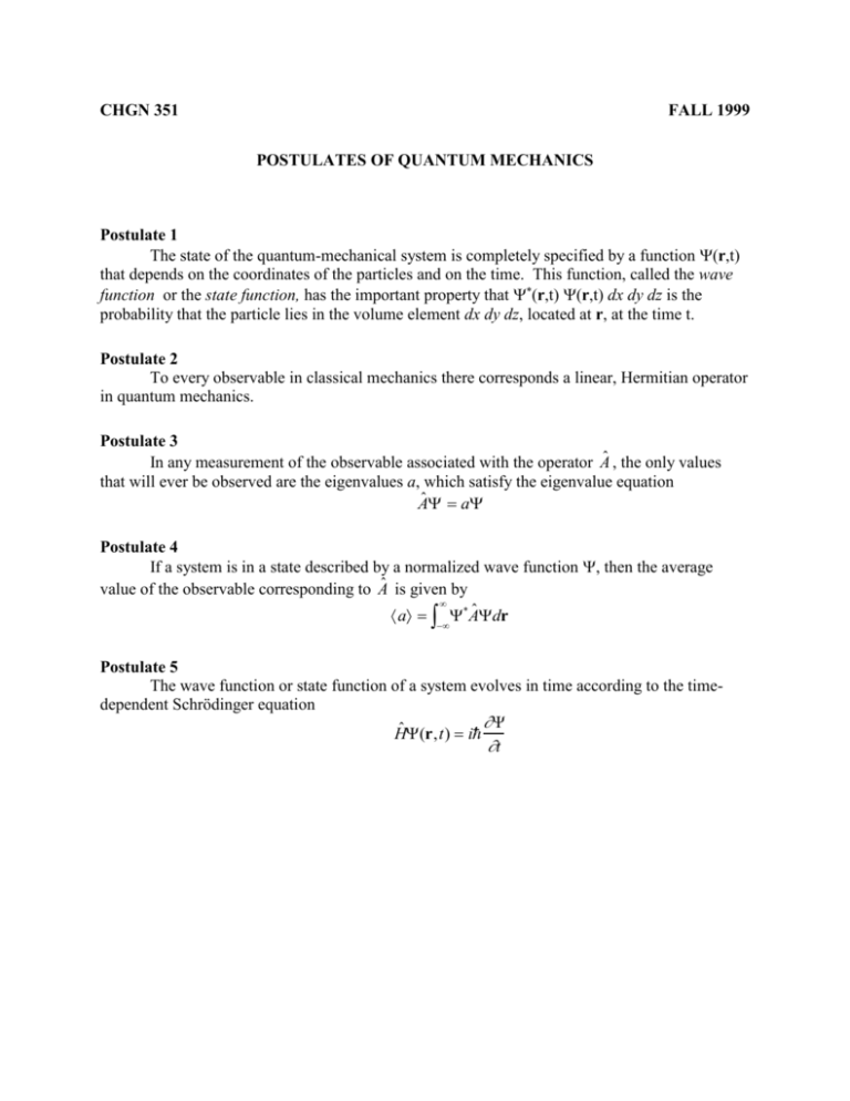
Postulate 1
The state of the quantum-mechanical system is completely specified by a function (r,t)
that depends on the coordinates of the particles and on the time. This function, called the wave
function or the state function, has the important property that *(r,t) (r,t) dx dy dz is the
probability that the particle lies in the volume element dx dy dz, located at r, at the time t.
Postulate 2
To every observable in classical mechanics there corresponds a linear, Hermitian operator
in quantum mechanics.
Postulate 3
In any measurement of the observable associated with the operator Aˆ , the only values
that will ever be observed are the eigenvalues a, which satisfy the eigenvalue equation
Aˆ   a
Postulate 4
If a system is in a state described by a normalized wave function , then the average
value of the observable corresponding to Aˆ is given by

a   Aˆ dr


Postulate 5
The wave function or state function of a system evolves in time according to the timedependent Schrödinger equation

Hˆ (r,t)  i
t
CHGN 351
FALL 1999
TIME-DEPENDENCE OF THE WAVEFUNCTION
From the postulates of QM, we find that a system is completely specified by its
wavefunction (r,t). This function satisfies the Schrödinger equation (the equation of motion
for the wavefunction) which in its similarity to the classical wave equation, can be solved by
similar methods. These are :
1) Separation of variables leading to the discovery of certain solutions of the product
form
(r,t) = (r) T(t)
T(t) specifies the time-dependence of the spatial function (r). The spatial part of the
separated equation is in fact the time-dependent Schrödinger Equation , and so the (r)
are the eigenfunctions of the Hamiltonian, and are the energy eigenstates, or stationary
states.
2) The requirement of boundary conditions limits the possible solutions (r) --sometimes
leading to discrete possible solutions (r), which can then be labeled by a “quantum
number” n, i.e., the solutions form a set {n(r)}
3) The property that the set of all possible solutions {n(r)} form an orthonormal basis
for any arbitrary function f(r) satisfying the given boundary conditions. In particular,
one can write
f(r) = n cn n(r)
Since the {n(r)} are an orthonormal basis, the coefficient cn for the component n(r) can
be determined by taking the projection of f(r) on that component, that is
cn =  f(r) n(r) dr
4) The time-dependence of a function initially (at t=0) set to be f(r) can then be solved by
the linear combination of the time varying n(r) Tn(t), that is
f(r,t) = n cn n(r) Tn(t)
Note how the last equation reduces to the above equation for f(r) when Tn(t=0) = 1.
CHGN 351
FALL 1999
MAKING MEASUREMENTS IN QUANTUM MECHANICS
As indicated above, the wavefunction need not be one of the stationary states but can be
any function satisfying constraints such as normalizability and continuity. Nonetheless, it can be
decomposed into a linear combination (or linear “superposition”) of the stationary states.
However, the stationary states, while a special basis because of their role in determining timedependence, are not the only possible basis. In fact, the eigenfunctions n(r) of any operator Aˆ
corresponding to a measurement of a real quantity (which in fact is equivalent to saying that Aˆ is
Hermitian) will form an orthonormal basis. Hence any (normalizable, continuous, and otherwise
observing the boundary conditions) spatial wavefunction (r) can be written as the linear
superpostion
(r) = n cn n(r)
(Note the coefficients cn are not the same as the “cn” used above for the stationary states.) Recall
that we have
Aˆ  n (r)  an n (r)
where the an are the only values that can be observed for the operator Aˆ .
We can then use Postulate 4 to determine the physical meanings of the coefficients cn :
If a system is in a state described by a normalized wave function , then the average
value of the observable corresponding to Aˆ is given by

a   Aˆ dr


The wavefunction  can then be decomposed in terms of the eigenstates of Aˆ :
a    cm*  *m (r) Aˆ  c n n (r)dr
m

c c a 
*
m n n
m ,n

c
n
2
n
*
m
(r) n (r)dr   c*m cn an m, n
m,n
an
n
Thus we see that the |cn|2 represent the weight of the possible observable values an , where
the above sum represents a weighted average over outcomes. Moreover, the |cn|2 represent a
valid normalized weight distribution, since it can be shown from the normalization condition on
(r) that
n |cn|2 = 1