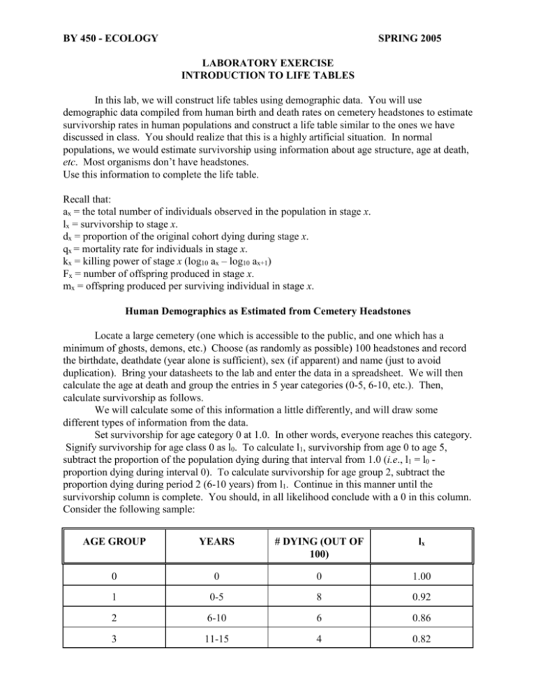
BY 450 - ECOLOGY
SPRING 2005
LABORATORY EXERCISE
INTRODUCTION TO LIFE TABLES
In this lab, we will construct life tables using demographic data. You will use
demographic data compiled from human birth and death rates on cemetery headstones to estimate
survivorship rates in human populations and construct a life table similar to the ones we have
discussed in class. You should realize that this is a highly artificial situation. In normal
populations, we would estimate survivorship using information about age structure, age at death,
etc. Most organisms don’t have headstones.
Use this information to complete the life table.
Recall that:
ax = the total number of individuals observed in the population in stage x.
lx = survivorship to stage x.
dx = proportion of the original cohort dying during stage x.
qx = mortality rate for individuals in stage x.
kx = killing power of stage x (log10 ax – log10 ax+1)
Fx = number of offspring produced in stage x.
mx = offspring produced per surviving individual in stage x.
Human Demographics as Estimated from Cemetery Headstones
Locate a large cemetery (one which is accessible to the public, and one which has a
minimum of ghosts, demons, etc.) Choose (as randomly as possible) 100 headstones and record
the birthdate, deathdate (year alone is sufficient), sex (if apparent) and name (just to avoid
duplication). Bring your datasheets to the lab and enter the data in a spreadsheet. We will then
calculate the age at death and group the entries in 5 year categories (0-5, 6-10, etc.). Then,
calculate survivorship as follows.
We will calculate some of this information a little differently, and will draw some
different types of information from the data.
Set survivorship for age category 0 at 1.0. In other words, everyone reaches this category.
Signify survivorship for age class 0 as l0. To calculate l1, survivorship from age 0 to age 5,
subtract the proportion of the population dying during that interval from 1.0 (i.e., l1 = l0 proportion dying during interval 0). To calculate survivorship for age group 2, subtract the
proportion dying during period 2 (6-10 years) from l1. Continue in this manner until the
survivorship column is complete. You should, in all likelihood conclude with a 0 in this column.
Consider the following sample:
AGE GROUP
YEARS
# DYING (OUT OF
100)
lx
0
0
0
1.00
1
0-5
8
0.92
2
6-10
6
0.86
3
11-15
4
0.82
At this point, lx may be viewed as the probability that an individual will survive to the end of the
xth interval.
We will now calculate the average life expectancy remaining to an individual at each age
interval. To do this, first determine the average survivorship for overlapping age intervals, Lx,
from age x to age w:
l x  l x 1
2
Lx 
Add this column to your life table. Sum these (it’s easiest to start from the bottom of the table
and work upward) and place the results in the Lx column. Now divide Lx by lx for each age
interval to determine life expectancy (ex). You may want to go ahead and multiply this by five to
convert from age intervals to years. Remember, each of your intervals represents five years.
Now, use the following fecundity schedule (number of female birth per five years per
female) to complete the life table.
AGE
0-10
11-15
16-20
21-25
26-30
31-35
36-40
41-45
46-50
51+
mx
0.000
0.002
0.166
0.424
0.348
0.193
0.094
0.026
0.002
0.000
These fecundity values are from the 1940's, and have no doubt changed over time. They should,
however, serve well for our purposes.
Now, add another column to the life table, lxmx. For this calculation, assume that your
data are good estimates of female survivorship. Realize that this column is calculating the
contribution of an individual female to population growth and utilizes information both about
survivorship to a particular age and fecundity during that age interval.
Calculate R0, the replacement rate, as:
w
R 0 = l x m x
x=0
and G, the generation interval as:
w
 xl
G=
x
mx
x=0
R0
and r, the intrinsic rate of population growth as:
r=
lnR 0
G
When calculating these intervals, remember that your data were analyzed in five-year increments,
so your intervals must be multiplied by 5 to equate to years. The same applies to life expectancy.
Using the methods above, complete the following life table for your human survivorship
data. Then, use your newly acquired knowledge to complete the following.
1. Use EXCEL to produce a surivorship curve and attach it to this lab report. Comment on
the type of survivorship curve observed. At what age does median life expectancy (lx = 0.50)
occur?
2. Can you make any predictions about human population growth from your data? If this were a
representative sample, is human population growing, declining, or remaining stable. Based on
your knowledge, does your data model the real world?
3. How many years are between generations in your data? Does this seem to be representative?
4. How might your data differ if your limited your observations to headstones for people born
before 1850? What other limitations can you suggest to this technique?
Number Dying
Interval
0
0
0
1
0-5
0
2
6-10
0
3
11-15
.002
4
16-20
.166
5
21-25
.424
6
26-30
.348
7
31-35
.193
8
36-40
.094
9
41-45
.026
10
46-50
.002
11
51-55
0
12
56-60
0
13
61-65
0
14
66-70
0
15
71-75
0
16
76-80
0
17
81-85
0
18
86-90
0
19
91-95
0
20
96-100
0
R0 = ________________________________
G = ________________________________
r = ________________________________
lx
Lx
 Lx
Age
ex
mx
lxmx
xlxmx
NAME
1
2
3
4
5
6
7
8
9
10
11
12
13
14
15
16
17
18
19
20
DATASHEET FOR HUMAN LIFE TABLE
SEX
BIRTH YEAR
YEAR OF DEATH
AGE AT DEATH