Supporting Information to
Fluorescence quantum yield and photochemistry of bacteriophytochrome constructs
K.C. Toh, Emina A. Stojković, Ivo H.M. van Stokkum, Keith Moffat, John T.M Kennis
Model based data analysis
The aim of data analysis is to obtain a model-based description of the full data set in
terms of a model containing a small number of precisely estimated parameters, of which
the rate constants and spectra are the most relevant. The basic ingredient of kinetic
models, namely the exponential decays, will be described first, followed by use of these
ingredients for global and target analysis1-3 of the full data. Our main assumption is that
the time and wavelength properties of the system of interest are separable, which means
that spectra of species or states are constant. For details on parameter estimation
techniques the reader is referred to1-4. Software issues are discussed in5.
A. Modeling an exponential decay
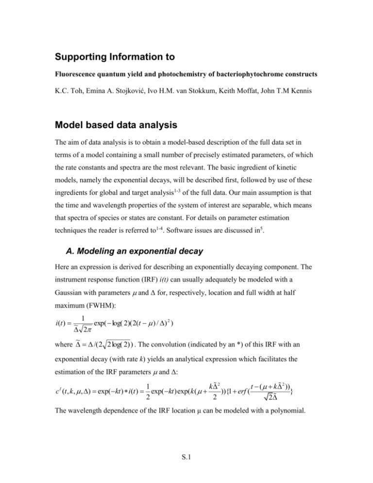
Here an expression is derived for describing an exponentially decaying component. The
instrument response function (IRF) i(t) can usually adequately be modeled with a
Gaussian with parameters  and Δ for, respectively, location and full width at half
maximum (FWHM):
1
i (t )  ~
exp(  log( 2)( 2(t   ) / ) 2 )
 2
~
where    /( 2 2 log( 2) ) . The convolution (indicated by an *) of this IRF with an
exponential decay (with rate k) yields an analytical expression which facilitates the
estimation of the IRF parameters  and Δ:
1
k 2
t  (   k  2 ))
c I (t , k ,  , )  exp(kt )  i(t )  exp(kt )exp(k (  
)){1  erf (
}
2
2
2
The wavelength dependence of the IRF location μ can be modeled with a polynomial.
S.1
jmax
 ( )     a j (  c ) j
c
j 1
Typically, a parabola is adequate and the order of this polynomial ( jmax ) is two. The
reference wavelength c is usually at the center of the spectrograph.
B. Global and target analysis
The basis of global analysis is the superposition principle, which states that the measured
data  (t ,  ) result from a superposition of the spectral properties  l ( ) of the
components present in the system of interest weighted by their concentration cl (t ) .
 (t ,  ) 
ncomp
 c (t ) ( )
l 1
l
l
The cl (t ) of all ncomp components are described by a compartmental model that consists
of first-order differential equations, with as solution sums of exponential decays. We
consider three types of compartmental models: (1) a model with components decaying
monoexponentially in parallel, which yields Decay Associated Difference Spectra
(DADS), (2) a sequential model with increasing lifetimes, also called an unbranched
unidirectional model6, which yields Evolution Associated Difference Spectra (EADS),
and (3) a full compartmental scheme which may include possible branchings and
equilibria, which yields Species Associated Difference Spectra (SADS). The last is most
often referred to as target analysis, where the target is the proposed kinetic scheme,
including possible spectral assumptions. In this paper we did not attempt a target
analysis. Instead, throughout the manuscript, the EADS are shown in the main text and
the corresponding DADS are shown in the Supporting Information.
(1) With parallel decaying components the model reads
 (t ,  ) 
ncomp
 c (k ) DADS ( )
I
l 1
l
l
The DADS thus represent the estimated amplitudes of the above defined exponential
decays c I ( kl ) . When the system consists of parallel decaying components the DADS are
true species difference spectra. In all other cases, they are interpreted as a weighted sum
(with both positive and negative contributions) of true species difference spectra.
S.2
(2)
A sequential model reads
 (t ,  ) 
ncomp
c
l 1
II
l
EADSl ( )
where each concentration is a linear combination of the exponential decays,
l
clII   b jl c I (kl ) , and the amplitudes6 b jl are given by b11  1 and for j  l :
j 1
l 1
b jl   km /
m 1
l

n 1, n  j
(kn  k j )
When the system consists of sequentially decaying components 1  2  ...  ncomp the
EADS are true species difference spectra. In all other cases, they are interpreted as a
weighted sum (with only positive contributions) of true species difference spectra.
Equivalence of the parallel and the sequential model
It is important to note that the fit is identical when using a parallel or a sequential model.
Both the estimated lifetimes and the residuals from the fit are identical. This can be
demonstrated as follows. Since the concentrations of the sequential model are a linear
combination of the exponential decays we can write for the matrix of concentrations
(where column l corresponds to component l)
C II  C I B
where the upper triangular matrix B contains the elements b jl defined above.
Furthermore, in matrix notation the parallel model reads
  C I DADS T
where DADS T is the transpose of the matrix that contains the DADS of component l in
column l. Likewise, in matrix notation the sequential model reads
  C II EADS T
Combining these three equations we obtain the relations
DADS  EADS  BT
EADS  DADS  B T
where the coefficients of the lower triangular matrix B T are given by b1l 1  1  b1l T and
for j  l :
S.3
j 1
b jl1  
n 1
( k n  kl )
 bljT
kn
Thus the DADS are linear combinations of the EADS, and vice versa. Thus, the lth
EADS is a linear combination of the lth and following DADS. In particular, the first
EADS, which corresponds to the time zero difference spectrum, is the sum of all DADS;
and the final EADS is proportional to the final DADS.
In systems where photophysical and photochemical processes occur the sequential model
with increasing lifetimes provides a convenient way to visualize the evolution of the
(excited and intermediate) states of the system. Therefore, the EADS are shown in the
main text and the corresponding DADS are shown in the Supporting Information.
References
(1)
Holzwarth, A. R. Data Analysis of Time-Resolved Measurements. In
Biophysical Techniques in Photosynthesis; Amesz, J., Hoff, A. J., Eds.; Kluwer:
Dordrecht, The Netherlands, 1996; pp 75.
(2)
van Stokkum, I. H. M.; Larsen, D. S.; van Grondelle, R. Biochimica Et
Biophysica Acta-Bioenergetics 2004, 1657, 82.
(3)
van Stokkum, I. H. M.; van Oort, B.; van Mourik, F.; Gobets, B.; van
Amerongen, H. (Sub)-Picosecond Spectral Evolution of Fluorescence Studied with a
Synchroscan Streak-Camera System and Target Analysis. In Biophysical Techniques in
Photosynthesis Vol. II; Aartsma, T. J., Matysik, J., Eds.; Springer: Dordrecht, The
Netherlands, 2008; pp 223.
(4)
van Stokkum, I. H. M. “Global and Target Analysis of Time-resolved
Spectra,” Department of Physics and Astronomy, Faculty of Sciences, Vrije Universiteit,
Amsterdam, The Netherlands, 2005.
(5)
van Stokkum, I. H. M.; Bal, H. E. “A Problem Solving Environment for
interactive modelling of multiway data”, 2006.
(6)
Nagle, J. F.; Parodi, L. A.; Lozier, R. H. Biophysical Journal 1982, 38,
161.
S.4