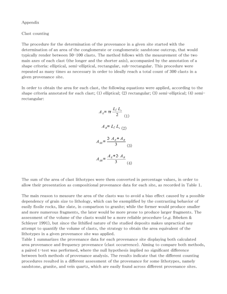
Appendix
Clast counting
The procedure for the determination of the provenance in a given site started with the
determination of an area of the conglomerate or conglomeratic sandstone outcrop, that would
typically render between 50-100 clasts. The method follows with the measurement of the two
main axes of each clast (the longer and the shorter axis), accompanied by the annotation of a
shape criteria: elliptical, semi-elliptical, rectangular, sub-rectangular. This procedure were
repeated as many times as necessary in order to ideally reach a total count of 300 clasts in a
given provenance site.
In order to obtain the area for each clast, the following equations were applied, according to the
shape criteria annotated for each clast; (1) elliptical; (2) rectangular; (3) semi-elliptical; (4) semirectangular:
A E= π⋅
Ll⋅ Ls
2 (1)
A R= Ll⋅ Ls (2)
A SE =
2⋅ A E + A R
3
(3)
A SR =
A E +2⋅ A R
3
(4)
The sum of the area of clast lithotypes were them converted in percentage values, in order to
allow their presentation as compositional provenance data for each site, as recorded in Table 1.
The main reason to measure the area of the clasts was to avoid a bias effect caused by a possible
dependency of grain size to lithology, which can be exemplified by the contrasting behavior of
easily fissile rocks, like slate, in comparison to granite; while the former would produce smaller
and more numerous fragments, the later would be more prone to produce larger fragments. The
assessment of the volume of the clasts would be a more reliable procedure (e.g. Ibbeken &
Schleyer 1991), but since the lithified nature of the studied deposits makes unpractical any
attempt to quantify the volume of clasts, the strategy to obtain the area equivalent of the
lithotypes in a given provenance site was applied.
Table 1 summarizes the provenance data for each provenance site displaying both calculated
area provenance and frequency provenance (clast occurrence). Aiming to compare both methods,
a paired t-test was performed, where the null hypothesis implied no significant difference
between both methods of provenance analysis. The results indicate that the different counting
procedures resulted in a different assessment of the provenance for some lithotypes, namely
sandstone, granite, and vein quartz, which are easily found across different provenance sites.
While most of the rock varieties found in the studied conglomerates did not bear a detectable
dependency between clast size and lithology, it is important to notice that the differences in the
counting methods were more sensible to lithotypes that have a tendency to produce larger and
less fissile clasts. This particularity suggests that simply recording the frequency of clasts would
probably result in an under representation of sedimentary and granitic sources to the basin fill.
These sources comprise an important share of the source rocks bordering the studied basin, thus
justifying the assessment of the provenance using methods that can compensate the bias caused
by the dependency between lithology and grain size.
Substitution of zero values
In order to make possible the multivariate statistical analysis of the provenance data (expressed
in percentage), the dataset needs to be converted to an unclosed data range, reached by the
application of logarithmic ratios to the dataset (Aitchison 1986). However, the existence of
compositional zeros (recorded when a given lithotype were not found in a provenance site) makes
unfeasible the application of logarithmic ratios. This caveat is avoided by the substitution of null
values by another defined value (Aitchison 1986, Martín-Fernandez et al. 2003).
Considering that the zero values found in the provenance dataset are rounded zeros, and not
absolute zeros (Martín-Fernández et al. 2003, Martín-Fernández & Thió-Henestrosa 2006), it
can be said that a zero value represents a possible existence of the component, however, below
the detection limit of the method. This way, in order to obtain the logarithmic ratio, a
multiplicative substitution method of imputation was chosen (Martín-Fernández et al. 2003),
presenting the advantage of preserving the covariance of the sample (in comparison to other
substitution methods).
However, instead of making use of a fixed value for the substitution of zeros, like 65% of the
detection limit, as proposed by Martín-Fernández et al. (2003) and Palarea-Albaladejo et al.
(2007), an alternative strategy was used, resulting in values below the detection limit of the
provenance analysis (in this case, a clast with 0,25 cm2), which were specific to each provenance
site.
In order to substitute zeros, the chosen value should have an area equivalent to the sample error
of each site, so that the imputed value would be statistically indistinguishable from zero in a
given population. In this way, the substitution of zeros is based in the sample error ε of each
observation equivalent to the true proportion p of the occurrence of a component present in the
counting of a population n, as follows:
ε= Z⋅
√
p⋅ (1− p)
n
(5)
Where Z is the value related to the probability that ε is equivalent to p.
Considering that each observation corresponds to the detection limit of the macroscopic
provenance analysis (i.e., a clast with 0.5 cm length for both axis), it can be said that every
square centimeter corresponds to four observations, so that:
n= A⋅ 4 (6)
Where n is the sample population and A corresponds to the total sum of the area of the
components recorded in a given provenance site. This approach ensures that every provenance
site have a particular value for the substitution of zero, which is related to the volume of
fragments found in the sedimentary deposit, thus being representative of possible source areas.
Inserting the equation (6) into equation (5), and using Z for a probability of 95%, the following
equation is obtained:
ε= 1,96⋅
√
p⋅ (1− p)
A⋅ 4 (7)
When ε = p, ε represents the least possible proportion of occurrence of a given component in
a provenance site, which is them used to substitute the zero values in the components of the
provenance analysis.
Following the substitution of zeros, the dataset is them normalized to assure a fixed total range
for the compositional dataset, subjecting every component that was not substituted by the ε
value obtained from equation (7) to the following equations:
C ' i = Ci⋅ (
100− E
)
100 (8)
E= ( ∑ x= ε)
x∈C
(9)
Where C'i corresponds to the normalized value of the component Ci and E represents the sum of
the error ε of every component in a sample space C that had the zero value substituted for the
ε error.
Once the dataset is free of zero values, it is ready for logarithmic transformation. As pointed out
by Pawlowsky-Glahn & Egozcue (2006), there are at least three types of transformation to
consider: alr – additive logarithmic ratio; ilr – isometric logarithmic ratio; and clr – centered
logarithmic ratio. In each of the transformations the composition of the sample is turned to a
vector. For alr and ilr the method of transformation result in vectors with one missing
component, while for clr the total number of components is preserved. In this way, the chosen
method for logarithmic transformation was the clr, which is essentially the logarithmic value of
the product of a component by the geometric mean of the components of a given sample, as
demonstrated in equation (10):
clr (x 1 , x 2 , ... , x n )= [ln
x1
1 , ln
( x 1∗ x 2∗ ...∗ x n)n
x2
1 , ... , ln
( x1∗ x 2∗ ...∗ x n ) n
xn
(x 1∗ x 2∗ ...∗ x n )
1
n
]
(10)
The clr method of transformation has the advantage of providing easier geologic interpretation of
the data, and is particularly functional in multivariate statistics (Pawlowsky-Glahn & Egozcue
2006). Once done the logarithmic transformation, the provenance dataset is ready for
multivariate statistical analysis.
References
AITCHISON, J. (1986) The statistical analysis of compositional data. Monographs on statistics
and applied Probability: Chapman & Hall, London, 416 p.
IBBEKEN, H. & SCHLEYER, R. (1991) Source and Sediment - A case study of provenance and
mass balance at an active plate margin (Calabria, southern Italy). Springer-Verlag, BerlinHeidelberg.
MARTÍN-FERNANDEZ, J.A. & THIÓ-HENESTROSA, S. (2006) Rounded zeros: some practical
aspects for compositional data. Geological Society Special Publication, 264, Geological Society of
London.
PALAREA-ALBALADEJO, J., MARTÍN-FERNANDEZ, J.A. & GOMEZ-GARCIA, J. (2007) A
parametric approach for dealing with compositional rounded zeros. Mathematical Geology, 39,
625-645.
PAWLOWSKY-GLAHN, V. & EGOZCUE, J. J. (2006) Compositional data and their analysis: an
introduction, Geological Society of London, Special Publications, 264 (1), 1-10.