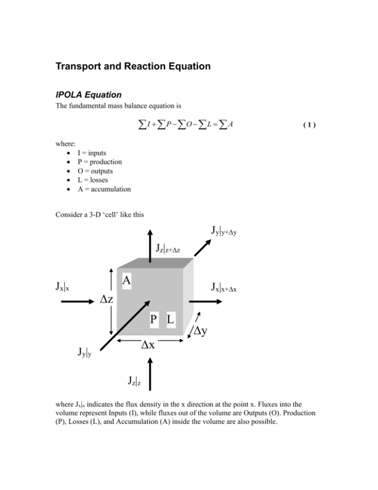
Transport and Reaction Equation
IPOLA Equation
The fundamental mass balance equation is
 I   P  O   L   A
(1)
where:
 I = inputs
 P = production
 O = outputs
 L = losses
 A = accumulation
Consider a 3-D ‘cell’ like this
Jy|y+y
Jz|z+z
A
Jx|x
Jx|x+x
z
P L
x
Jy|y
y
Jz|z
where Jx|x indicates the flux density in the x direction at the point x. Fluxes into the
volume represent Inputs (I), while fluxes out of the volume are Outputs (O). Production
(P), Losses (L), and Accumulation (A) inside the volume are also possible.
The cell can represent a small piece of many different things; it might represent a volume
of water in a pond, part of the atmosphere, a portion of an aquifer, or a block of steel.
Similarly, the flux density J might be a liquid flow, a heat (energy) flux, or a chemical
flux. Since our primary interest is in the movement of chemicals in the environment,
we’ll consider only the flux of chemical mass here. The approach has broad applicability
though.
Advective Flux Density
The mass flux (ML-2T-1) can consist of a number of components. First, there may be a
fluid (liquid or gas) flow with velocity v that carries along a mass of chemical. Let’s
consider just the x direction. In time t, a velocity v (at x) will sweep in a volume V = v|x
t y z. The volume swept out may be different because it depends on the velocity at x
+ x.
The chemical mass going in or out in time t depends on the fluid volume and the
concentration C in the fluid:
Mass/Time = Concentration x Volume/Time.
If we divide everything by the area of the inflow (or outflow) faces, we get the mass flux
density, which ends up being very simple:
Jx|x = C v
where C is concentration and v is the velocity at point x.
Diffusive/Dispersive Flux
A second possible contribution to Jx|x is diffusion or dispersion. We know from Fick’s
Law that the diffusive/dispersive flux density (in the x direction at point x) is
J x x  D
C
x
(2)
x
Similar expressions can be written for the diffusive/dispersive fluxes in the y and z
directions and at the other edges of the control volume.
Total Input/Output Fluxes
The advective and diffusive/dispersive fluxes can simply be added together to get the
totals. We’ll have one flux for each face of the control volume (6 altogether). Three (at
points x, y, and z) will be inputs and 3 (at x + x, y + y, and z + z) will be outputs:
Inputs
J x x  Cvx x  D
Jy
y
C
x
 Cv y  D
y
J z z  Cvz z  D
(3)
x
C
y
C
x
(4)
y
(5)
z
Outputs
Jx
Jy
Jz
x  x
 Cvx
y  y
 Cv y
z  z
 Cvz
x  x
y  y
z  z
D
C
x
x  x
C
y
y  y
C
z
z  z
D
D
(6)
(7)
(8)
Production and Losses
Production of a particular chemical species can be the result of a chemical reaction. For
example, nitrification of organic forms of nitrogen results in the production of nitrate
(NO3-). Losses can be due to radioactive decay for example.
We will consider two types of reactions that lead to production or losses. Zero order
reactions proceed at a constant rate, with chemical mass being produced or lost. The
reaction rate dC/dt = k0 (a constant) is given as M L-3 T-1 or mols L-3 T-1, i.e., per unit
volume and time. dC/dt < 0 indicates loss, while dC/dt > 0 indicates production. If we
multiply by the volume of our cell (xyz), we can get the total mass rate of loss or
production in the cell.
First order reactions are characterized by rates that depend on the concentration present.
For these reactions
C
  k1C
t
(9)
Accumulation
The rate of change of chemical mass in the control volume is CV/t where C is the
change in concentration over the time t. If we replace the volume V by xyz and use
small C and t, we can express the accumulation A in terms of the change in
concentration over time:
A
C
xyz
t
( 10 )
Putting it all together
Start with IPOLA:
 I   P  O   L   A
( 11 )
To get the total amounts coming in through a face we have to multiply the flux densities
by the area of the face (yz for the x direction, xz for the y direction, and xy for
the z direction).
The sum of the inputs is


C 
C
Cv

D

y

z

Cv y y  D
 xx

x x 
y




C 
 xz  Cvz z  D
 xy

x

z


y
( 12 )
and the sum of the outputs is

Cv x


Cv z

x  x
z  z
D
C
x
C
D
z



y

z

Cv y


x  x 

 xy
z  z 
IPOLA uses I – O, so we end up with
y  y
D
C
y

 xz 
y  y 

( 13 )



C 
C 
C 
 xz  Cv z z  D
Cv x x  D
 yz  Cv y y  D
 xy 
x x 
y y 
x z 








C
C
Cv x x  x  D


y

z

Cv

D

x

z



y y  y

x x  x 
y y  y 








C
Cv z z  z  D

 xy
z z  z 


( 14 )
We can simplify this by collecting terms that have identical factors:

Cv x x  Cv x

x  x

 Cv y  Cv y
y


 Cv z z  Cv z

D
y  y
z  z
C
C
D
x x
x
D
D

 yz
x  x 
C
C
D
y y
y
C
C
D
x z
z

 xz

y  y 
( 15 )

 xy
z  z 
That is I – O. Let’s add the P (or L) and A terms:


C
C
D
Cv x x  Cv x x  x  D
 yz
x x
x x  x 



C
C
 Cv y  Cv y
D
D
 xz
y
y  y
y y
y y  y 



C
C
 Cv z z  Cv z z  z  D
D
 xy
x z
z z  z 

C
 k 0 xyz  k1Cxyz 
xyz
t
Now divide everything by xyz.
( 16 )

Cv x x  Cv x

x  x
D
C
C
D
x x
x


x  x 
x

Cv y y  Cv y



Cv z z  Cv z

 k 0  k1C 
y  y
D
C
C
D
y y
y


y  y 

y
z  z
D
C
C
D
x z
z
( 17 )


z  z 
z
C
t
Look at the first part of the first term:
Cv x x  Cv x
x  x
( 18 )
x
If we write this as

 Cv x
x  x
 Cv x
x

x
( 19 )
we see that it is the negative of the slope (gradient) of Cv:
Cv|x
Cv|x+x
x
x +x
Hence, for infinitesimal x, we can write it as the derivative

 Cv 
t
( 20 )
Similarly, the second part of the first term is

C
C
D
 D
x x
x

x
or


x  x 
( 21 )
 C
D
 x
D
x  x
C 

x x 
( 22 )
x
∂C/∂x|x
x
∂C/∂x|x+x
x +x
We are taking the gradients of the gradients, and if we shrink x and y to differential
size we have
 C 
 D x 
 2C

D 2
x
x
( 23 )
Of course, there are similar expressions for the y and z directions. Using them in ( 17 )
yields
 Cvx  Cv y  Cvz  
  2C  2C  2C 
C
  D 2  2  2   k 0  k1C 
 


y
z 
t
y
z 
 x
 x
( 24 )
This is the advection diffusion reaction equation. It can take various forms depending on
the details of the system, but overall it will have a form similar to ( 24 ).
In one dimension with constant flow velocity ( 24 ) simplifies to
C
 2C
C
v
 D 2  k 0  k1C 
x
t
x
( 25 )
This can often be used if the coordinate system is carefully chosen.
There are some analytical solutions of this equation but for many situations numerical
solutions are required.