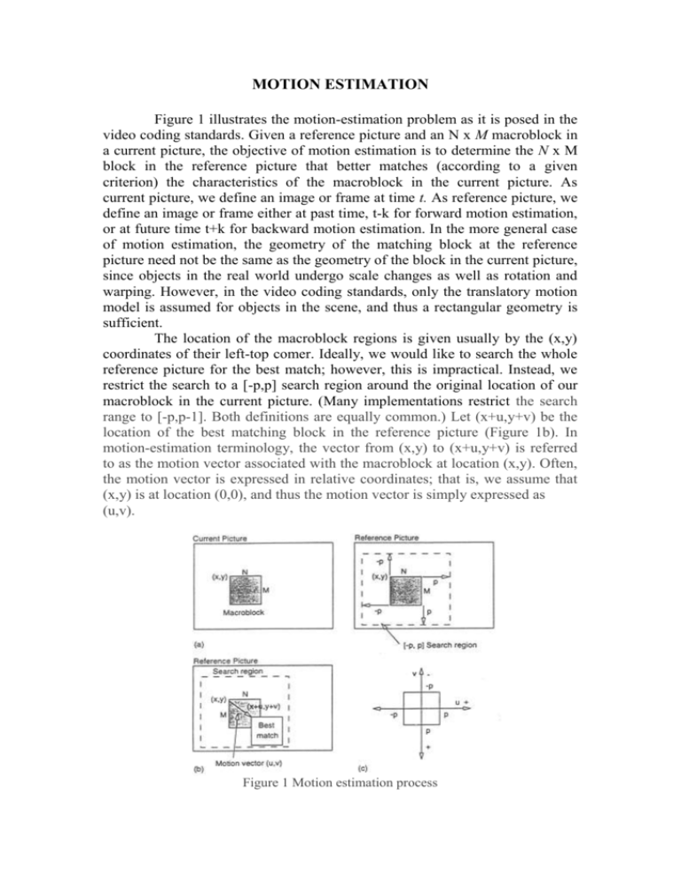
MOTION ESTIMATION
Figure 1 illustrates the motion-estimation problem as it is posed in the
video coding standards. Given a reference picture and an N x M macroblock in
a current picture, the objective of motion estimation is to determine the N x M
block in the reference picture that better matches (according to a given
criterion) the characteristics of the macroblock in the current picture. As
current picture, we define an image or frame at time t. As reference picture, we
define an image or frame either at past time, t-k for forward motion estimation,
or at future time t+k for backward motion estimation. In the more general case
of motion estimation, the geometry of the matching block at the reference
picture need not be the same as the geometry of the block in the current picture,
since objects in the real world undergo scale changes as well as rotation and
warping. However, in the video coding standards, only the translatory motion
model is assumed for objects in the scene, and thus a rectangular geometry is
sufficient.
The location of the macroblock regions is given usually by the (x,y)
coordinates of their left-top comer. Ideally, we would like to search the whole
reference picture for the best match; however, this is impractical. Instead, we
restrict the search to a [-p,p] search region around the original location of our
macroblock in the current picture. (Many implementations restrict the search
range to [-p,p-1]. Both definitions are equally common.) Let (x+u,y+v) be the
location of the best matching block in the reference picture (Figure 1b). In
motion-estimation terminology, the vector from (x,y) to (x+u,y+v) is referred
to as the motion vector associated with the macroblock at location (x,y). Often,
the motion vector is expressed in relative coordinates; that is, we assume that
(x,y) is at location (0,0), and thus the motion vector is simply expressed as
(u,v).
Figure 1 Motion estimation process
Note that, our assumption for a common displacement (u,v) for all
pixels in the macroblock implies that we are essentially imposing a local
smoothness constraint on the motion vector field. The local smoothness
constraint is only satisfied for small macroblock sizes. The choice of the
dimensions of the macroblock is the result of tradeoffs among three conflicting
requirements. Specifically,
1. small values for N and M (from four to eight) are preferable, since the
smoothness constraint would be easily met at this resolution;
2. small values for N and M reduce the reliability of the motion vector (u, v),
since few pixels participate in the matching process; and
3. fast algorithms for finding motion vectors are more efficient for larger
values of Nand M.
In the video coding standards, N = M = 16.
The coordinate system associated with the motion vector is shown in Figure 1c.
For the search region shown in Figure 4.11a, -p≤u≤p and -p≤v≤p. For broadcast
TV, good performance is obtained at p = 15 and at p = 63 for sporting events
(high motion).
Parallel Hierarchical One-Dimensional Search (PHODS)
The phods search algorithm is as follows:
1. For a [-p,p] search region as shown in Figure 4.11, let S  2 |log p| and set
the origin of the search space at search location (0, 0). Denote the origin
as (di,dj).
2. In parallel, compute the
 i-axis local minimum: Among the three locations (di-S,dj), (di,dj),
(di+S,dj) find the location that yields the smallest MAE. Set di to the
i coordinate of this location.
 j-axis local minimum: Among the three locations , find the location
that yields the smallest MAE. Set dj to the j coordinate of this
location. Set S = S/2.
Repeat step 2, until S = 0. The final (di,dj) is the motion vector that yields the
best match for the macroblock in the current picture.
This procedure is illustrated in Figure 2 for the case of p=7.
Figure 2 Example of Phods strategy
First, S = 4.
1. In the first step, for the i-axis minimum, we compute MAE for the three
search locations labeled xl. Assume that the minimum is obtained at i =
0. In parallel, we compute the j-axis minimum using search locations
labeled yl. Assume that the MAE minimum is obtained at y = 0. Thus
the new origin is again (0,0).
2. The spacing is reduced to 2. The i-axis minimum is obtained from the
search locations centered at the origin obtained in the previous step, and
these search locations are labeled x2. Assume that the MAE minimum is
attained at i = -2. For the j-axis minimum, as in the i-axis case, we
compute MAE for the j-axis search locations labeled y2. Assume the
MAE minimum is attained at j = 2. Thus the new search origin is (-2,2).
3. For this step, S = 1, and the minimum MAE along the i-axis is
determined from MAE computations at search locations labeled x3. We
can determine in parallel the minimum MAE along the j-axis by
computing the MAE at locations labeled yZ. Assume that the MAE
minimum along the i- and j-axis is attained at (-3,1). Since S = 1 at the
start of this step, no further reduction in spacing is possible, and this
terminates the search algorithm. We declare (-3,1) as the location
yielding the smallest MAE and therefore the motion vector for the
macroblock in the current picture.