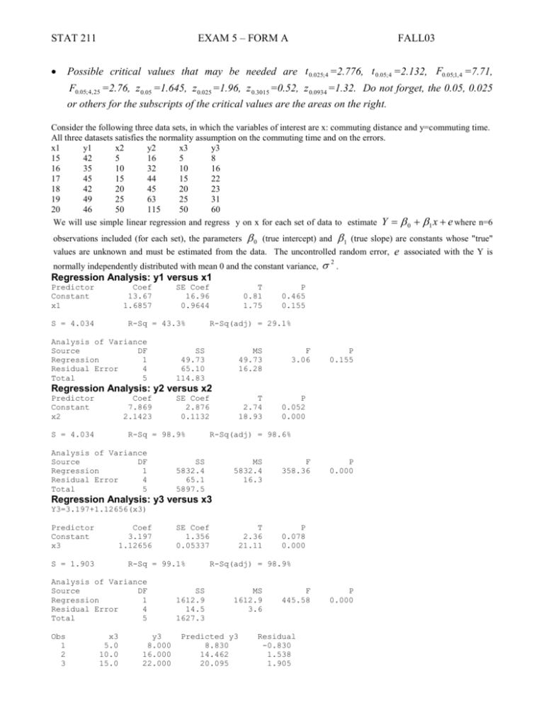
EXAM 5 – FORM A
STAT 211

FALL03
Possible critical values that may be needed are t 0.025; 4 =2.776, t 0.05; 4 =2.132, F0.05;1, 4 =7.71,
F0.05; 4, 25 =2.76, z 0.05 =1.645, z 0.025 =1.96, z 0.3015 =0.52, z 0.0934 =1.32. Do not forget, the 0.05, 0.025
or others for the subscripts of the critical values are the areas on the right.
Consider the following three data sets, in which the variables of interest are x: commuting distance and y=commuting time.
All three datasets satisfies the normality assumption on the commuting time and on the errors.
x1
y1
x2
y2
x3
y3
15
42
5
16
5
8
16
35
10
32
10
16
17
45
15
44
15
22
18
42
20
45
20
23
19
49
25
63
25
31
20
46
50
115
50
60
We will use simple linear regression and regress y on x for each set of data to estimate Y   0   1 x  e where n=6
observations included (for each set), the parameters
0
(true intercept) and
1
(true slope) are constants whose "true"
values are unknown and must be estimated from the data. The uncontrolled random error,
normally independently distributed with mean 0 and the constant variance,
 .
2
Regression Analysis: y1 versus x1
Predictor
Constant
x1
Coef
13.67
1.6857
S = 4.034
SE Coef
16.96
0.9644
R-Sq = 43.3%
T
0.81
1.75
Analysis of Variance
Source
DF
Regression
1
Residual Error
4
Total
5
P
0.465
0.155
R-Sq(adj) = 29.1%
SS
49.73
65.10
114.83
MS
49.73
16.28
F
3.06
P
0.155
Regression Analysis: y2 versus x2
Predictor
Constant
x2
Coef
7.869
2.1423
S = 4.034
SE Coef
2.876
0.1132
R-Sq = 98.9%
Analysis of Variance
Source
DF
Regression
1
Residual Error
4
Total
5
T
2.74
18.93
P
0.052
0.000
R-Sq(adj) = 98.6%
SS
5832.4
65.1
5897.5
MS
5832.4
16.3
F
358.36
P
0.000
Regression Analysis: y3 versus x3
Y3=3.197+1.12656(x3)
Predictor
Constant
x3
Coef
3.197
1.12656
S = 1.903
R-Sq = 99.1%
Analysis of Variance
Source
DF
Regression
1
Residual Error
4
Total
5
Obs
1
2
3
SE Coef
1.356
0.05337
x3
5.0
10.0
15.0
y3
8.000
16.000
22.000
SS
1612.9
14.5
1627.3
T
2.36
21.11
P
0.078
0.000
R-Sq(adj) = 98.9%
MS
1612.9
3.6
Predicted y3
8.830
14.462
20.095
F
445.58
Residual
-0.830
1.538
1.905
P
0.000
e associated with the Y is
EXAM 5 – FORM A
STAT 211
4
5
6
20.0
25.0
50.0
23.000
31.000
60.000
25.728
31.361
59.525
FALL03
-2.728
-0.361
0.475
Answer the following 11 questions using this information.
1) In which of those three datasets simple linear regression would be least effective? (Use =0.05)
(a) 1
because of very low rsquare and failing to reject H0: slope is zero (no relationship)
(b) 2
(c) 3
(d) both 1 and 2
(e) both 2 and 3
2) What change in y3 can be expected when x3 decreases by 100 units?
(a) -319.7
(b) -112.656
=-100(slope)=-100(1.12656) because of decrease, it becomes negative.
(c) -1.12656
(d) 1.12656
(e) 112.656
3) I have not attached the output for the Pearson’s correlation but you have enough information to compute it using the
outputs. Which of the following is the Pearson’s correlation coefficient between x3 and y3?
(a) 0.982
(b) 0.991
(c) 0.996
=r= R  0.991 only in simple linear regression. It is positive because of positive slope
(d) I do not have enough information on any of those outputs to compute it
2
4) Which of the following is the point estimate for the constant standard deviation in regressing y3 on x3?
(a) 1.897
(b) 1.903
(c) 3.6
(d) 14.5
=s=
MSE  3.6
5) When you look at the output of regressing y3 on x3, which of the following can you say about the intercept of the
regression equation?
(a) The equation definitely needs an intercept using 0.05 significance
(b) Testing the null hypothesis of no intercept, we fail to reject the null hypothesis using 0.05 significance. We
may want to fit without the intercept and see if it is a better fit
since the P-value=0.078 > =0.05, we fail to reject H0
(c) Testing the null hypothesis of no intercept, we reject the null hypothesis using 0.05 significance. We do not need to
fit without the intercept and see if it is a better fit
6) Which of the following is a possible relationship between x1 and y1? (Use α=0.05 and base your decision on testing
the slope)
(a) They are positively related
(b) They are negatively related
(c) There is no apparent relationship
the P-value=0.155 > α=0.05, then fail to reject H 0 : 1  0
7) What is the corresponding residual in the regression analysis of regressing y3 on x3 when x3=10?
(a) -6
(b) 1.54
when x3=10, y3=16 and predicted y3=14.462 then residual=y3-predicted y3
(c) There is no way to compute it with the given information
8) Suppose =1.93 and consider x3=10, what is P(Y3>17)?
(a) 0.0934
P(Y3>17)=P(Z>(17-14.462)/1.93)=P(Z>1.32)
(b) 0.3015
(c) 0.5200
(d) 0.6985
EXAM 5 – FORM A
STAT 211
FALL03
(e) 0.9066
9) Which of the following is the 95% confidence interval for the expected change in y3 associated with a 1 unit increase
in x3?
(a) (0.9784 , 1.2747)
C.I for the slope: 1.12656 t0.025;4 (0.05337) where t0.025;4 =2.776
(b) (1.0118 , 1.2394)
(c) (1.0219 , 1.2312)
(d) I do not have enough information to compute it.
10) Would you feel comfortable predicting y3 when x3=92 using the fitted regression equation?
(a) Of course, the predicted y3 is 119.6322
(b) Not at all
93 does not fall into the range of x3’s
11) How much of the total variation for y2 is explained by the model relationship with x2?
(a) 2.1423%
(b) 16.3%
(c) 18.93%
(d) 98.9%
is the rsquare by definition
(e) Cannot be determined with the given information
Numerous factors contribute to the smooth running of an electric motor. In particular, it is desirable to keep motor noise
and vibration to a minimum. To study the effect that the brand of bearing has on motor vibration, five different motor
bearing brands (each with true mean,  i     i where  is the overall mean and  i is the ith treatment effect ,
i=1,2,3,4,5) were examined by installing each type of bearing on different random samples of six motors. The amount of
motor vibration ( X ij in microns) was recorded when each of the 30 motors was running. We will model this data by
single factor ANOVA where X ij 
   i   ij .  ij ’s are errors which are normally distributed with mean, 0 and the
constant variance,  .
2
Analysis of Variance for vibration
Source
DF
SS
MS
Brand
4
30.855
7.714
Error
25
22.838
0.914
Total
29
53.694
Level
1
2
3
4
5
N
6
6
6
6
6
Mean
13.683
15.950
13.667
14.733
13.083
Pooled StDev =
Tukey's pairwise
Family error
Individual error
Critical value =
StDev
1.194
1.167
0.816
0.940
0.479
0.956
F
8.44
P
0.000
Individual 95% CIs For Mean
Based on Pooled StDev
---------+---------+---------+------(----*-----)
(----*-----)
(----*----)
(----*-----)
(----*-----)
---------+---------+---------+------13.5
15.0
16.5
comparisons
rate = 0.0500
rate = 0.00706
4.15
Intervals for (column level mean) - (row level mean)
1
2
3
4
2
-3.8860
-0.6473
3
-1.6027
1.6360
0.6640
3.9027
4
-2.6693
0.5693
-0.4027
2.8360
-2.6860
0.5527
EXAM 5 – FORM A
STAT 211
5
-1.0193
2.2193
1.2473
4.4860
-1.0360
2.2027
FALL03
0.0307
3.2693
Bartlett's Test (normal distribution)
Test Statistic: 4.097
P-Value
: 0.393
Answer the following 6 questions using this information.
12) Are there any significant differences between the true means of those five brands using 0.05 significance?
(a) Yes
Since the P-value=0 < =0.05 then reject H 0 : 1   2   3   4   5
(b) No
13) Look at the Tukey’s pairwise comparisons and tell me which of the following is the right conclusion using =0.05?
(a) I do not need to look at the Tukey’s pairwise comparisons because there are no differences between the true means
of those 5 brands.
(b) There are no significant differences between brand 1 and each of the others.
(c) There are no significant differences between brand 2 and each of the others.
(d) There are significant differences between brand 3 and brand 4
(e) There are significant differences between brand 4 and brand 5.
14) Which of the following is the point estimate of the 3rd brands effect?
(a) -0.5402
_
^
(b)
(c)
(d)
(e)
-0.5562
13.667
14.223
14.733

 3  x 3  x =13.667-14.2232 where 14.2232 is the overall sample mean
15) Which of the following is the point estimate for the constant standard deviation in analysis of variance?
(a) 0.914
^
(b) 0.956
=   MSE  0.914
(c) 7.714
(d) Unfortunately, constant variance assumption is not satisfied to compute the estimate using 0.05 significance.
16) I have found out brand 3 is not different than brand 4 and 5 when I look at the Tukey’s pairwise comparisons using
0.05 significance? I decided to compare the true average of brand 3 with the combined average of brands 4 and 5.
Which of the following should be the null hypothesis to test this?
(a)  3   4 and  3   5
3   4 and  4   5
(c)  3   4   5
(d) 2 3   4   5
(b)
17) For the test in question 16, I have computed the P-value as 0.6186 where =0.05. Are there significant differences
between the true average of brand 3 and the combined average of brands 4 and 5?
(a) Yes
(b) No
Since the P-value > , fail to reject H0: no differences. Conclude that there are no differences
18) You will have taken 5 exams this semester in STAT211. In one of the sections that I am teaching, each of the first two
exams are taken by 100 students but the remaining three exams are by 90 students each. We would examine the
significant differences between these 5 exams modeling with the single factor ANOVA. Which of the following would
be the error degrees of freedom?
(a) 4
(b) 85
(c) 95
STAT 211
(d) 185
(e) 465
EXAM 5 – FORM A
FALL03
There are total 2(100)+3(90)=470 students have taken all exams. df=n-I=470-5
19) Let’s say I have given you the boxplot and the normal probability plot of residuals to check the assumption of
normality for the analysis of variance. Boxplot indicates nonnormal residuals where the normal probability indicates
normally distributed residuals. Which of those you should use to see if the normality assumption is satisfied?
(a) Only boxplot
(b) Only normal probability plot
20) Which of the following is not correct?
(a) If the data is normally distributed we can use the Barttlett’s test to check the constant variance in different groups.
(b) If the data is continuous, we can use the Levene’s test to check the constant variance in different groups.
(c) If the data is not normally distributed, we can still use the Levene’s test to check the constant variance in
different groups for any other distribution.
Only for continuous distributions not the discrete distributions
(d) If the data is normally distributed and the constant variance assumption is satisfied, we can use the F-test in
analysis of variance to check the same true mean in different groups.
(e) If the data is normally distributed we can use the t-test for the slope or F-test in regression to check the relationship
between two numeric random variables