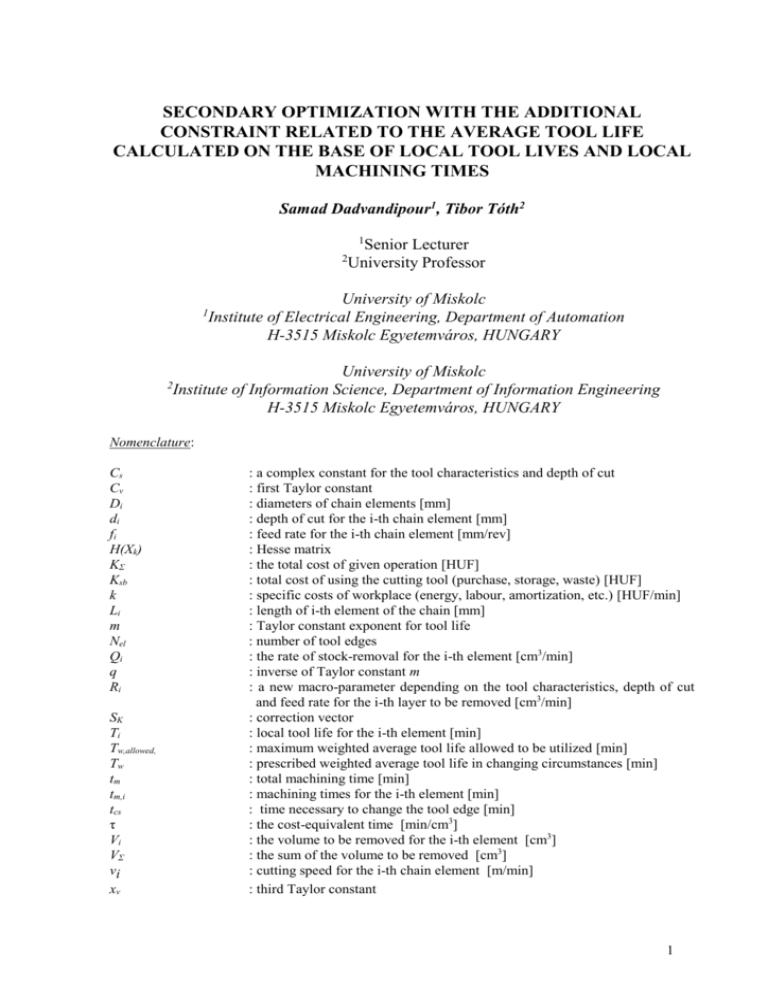
SECONDARY OPTIMIZATION WITH THE ADDITIONAL
CONSTRAINT RELATED TO THE AVERAGE TOOL LIFE
CALCULATED ON THE BASE OF LOCAL TOOL LIVES AND LOCAL
MACHINING TIMES
Samad Dadvandipour1, Tibor Tóth2
1
2
1
2
Senior Lecturer
University Professor
University of Miskolc
Institute of Electrical Engineering, Department of Automation
H-3515 Miskolc Egyetemváros, HUNGARY
University of Miskolc
Institute of Information Science, Department of Information Engineering
H-3515 Miskolc Egyetemváros, HUNGARY
Nomenclature:
Cs
Cv
Di
di
fi
H(Xk)
KΣ
Ksb
k
Li
m
Nel
Qi
q
Ri
SK
Ti
Tw,allowed,
Tw
tm
tm,i
tcs
τ
Vi
VΣ
vi
xv
: a complex constant for the tool characteristics and depth of cut
: first Taylor constant
: diameters of chain elements [mm]
: depth of cut for the i-th chain element [mm]
: feed rate for the i-th chain element [mm/rev]
: Hesse matrix
: the total cost of given operation [HUF]
: total cost of using the cutting tool (purchase, storage, waste) [HUF]
: specific costs of workplace (energy, labour, amortization, etc.) [HUF/min]
: length of i-th element of the chain [mm]
: Taylor constant exponent for tool life
: number of tool edges
: the rate of stock-removal for the i-th element [cm3/min]
: inverse of Taylor constant m
: a new macro-parameter depending on the tool characteristics, depth of cut
and feed rate for the i-th layer to be removed [cm3/min]
: correction vector
: local tool life for the i-th element [min]
: maximum weighted average tool life allowed to be utilized [min]
: prescribed weighted average tool life in changing circumstances [min]
: total machining time [min]
: machining times for the i-th element [min]
: time necessary to change the tool edge [min]
: the cost-equivalent time [min/cm3]
: the volume to be removed for the i-th element [cm3]
: the sum of the volume to be removed [cm3]
: cutting speed for the i-th chain element [m/min]
: third Taylor constant
1
yv
z
: second Taylor constant
: number of chain elements
: Lagrange-multiplier (constant)
: Lagrange function

 (Qi ,  )
 (Qi ,  )
: vector gradient of function (Qi ,  )
: Hungarian Forint.
HUF
Introduction
The new method of optimization works based on variable rate of stock removal
factor Qi (cm3/min). It aims at minimizing the total cost of the given operation KΣ
(HUF) as the objective function, [3, 4, 5, 2]. The constraint for this purpose is
maximum weighted average tool life that is allowed to be utilized Tw,allowed  Tw (min).
The macro- parameter R (cm3/min) is calculated based on the given input parameters
and Tw, allowed (min) is calculated on the base of local tool lives Ti [min] and machining
times tm,i (min). To find a suitable solution for the new optimization problem,
Lagrange-multiplier [1] method has been used. Applying Lagrange multiplier method
results in a new function denoted by  (Qi ,  ) . The derivation of function  (Qi ,  ) with
respect to the rate of the stock- removal factor Qi is the gradient vector of this function.
The gradient vector  (Qi ,  ) of function  (Qi ,  )
-linear system of
equations. The system has got N+1 unknowns and there is a need to apply a numerical
method to solve the problem for Qi and . The numerical solution based on
multidimensional Newton-method [1] has been applied to develop a program to
calculate the validity range of Lagrange-multiplier and the rates of stock removal
factors Qi too. After solving the system of non-linear equations for Qi and , the
optimised value of the total cost of the given operation KΣ (HUF) is obtained. The
process needs iteration steps by computer program, which turns the gradient vector
 (Qi ,  ) to zero. The new method of optimisation solves multidimensional problems
in cutting processes.
1. Summary of the mathematical model of the new optimization method
The general formula used for cost equivalent time function  (min/cm3) is as
follows: [3, 4, 5, 2]:
q 1
1 Q
   q
Q
R
[min/ cm3],
(1)
where the objective function is as follows:
 Vi
Qiq 1 

 [min/cm3]
K    K i  k   i Vi  k  
 Vi
q 
Ri 
i 1
i 1
i 1  Qi
z
z
z
 minimum.
(2)
2
The aim is to minimize the objective function (2) taking into consideration the
following conditional equation (3):
Tw, allowed  Tw
[min].
(3)
If we consider the maximum utilization of the weighted average tool life, which
is allowed to be utilized then we can have the following:
Tw, allowed  Tw  0
[min],
(4)
where:
z
Tw, allowed  Tw 
 T .t
i 1
z
t
i 1
Let us substitute Tw,
equation:
allowed
i
m ,i
[min].
(5)
m ,i
(5) in (4), and then we will have the following
z
 T .t
i 1
z
i
t
i 1
m ,i
 Tw  0
(6)
m ,i
Let us express machining times tm,i and local tool lives Ti in terms of rate of stock
removal factor Qi and macro-parameter Ri, then we will have the following:
t m,i  t m,i (Qi )
(7)
Ti  Ti (Qi , Ri )
(8)
Equation (7) may be considered in terms of Qi as follows:
t m ,i 
Vi
Qi
[min].
(9)
Let us also express Ti in terms of Qi using Taylorian tool life equation as follows:
1

m
C
Ti   xv vy v 
 di . fi .vi 
[min].
(10)
Let us express (10) as follows:
3
1

C
d . f m
Ti   xv vy v . i i 
 di . fi .vi di . fi 
[min].
(11)
As is known di fi vi = Qi , substituting this value of Qi in (11) we will have the
following equation:
 C .d 1 xv . fi1 y v
Ti   v i
Qi

1
m


[min].
(12)
[cm3/min].
(13)
m
(14)
Further more the macro-parameter Ri is as follows:
Ri  C s . f i1 yv
Where machining cost unit per minute is as follows:
Cs 
C v .d i1 xv
 K sb

 t cs 

 k .N el

We can express equation (13) as follows:
fi1 yv 
Ri
.
Cs
(15)
And (14) as follows:
 K

Cv .di1 xv  Cs  sb  tcs  .
 k.Nel

(16)
m
 K

For the sake of simplicity let us denote  sb  tcs  with A, then (16) turns to be as
 k .N el

follows:
 K

Cv .di1 xv  Cs  sb  tcs  .m  Cs A.m
 k.Nel

(17)
Let us substitute (15) and (17) in (12), then we will have the following:
 C . A m .Ri
Ti   s
 C s .Qi
 m1
.


(18)
4
After summarizing (18) we will get the following:
 A m .Ri
Ti  
 Qi
 m1
.


(19)
Am is a constant, then we may express (19) in terms of Qi and Ri as follows:
R  1
Ti  A  i . m
 Qi 
(20)
Let us substitute q = 1/m, then (20) will be as follows:
R 
Ti  A  i .q
 Qi 
(21)
Substituting (9) and (21) in conditional equation (6) we will get the following
equation:
q
 R  V
A  i  . i
i 1  Qi   Qi
z
 Vi 
 

i 1  Qi 
z


  T  0.
w
(22)
Let us apply Lagrange multipliers method to the objective function (2) and the
new conditional equation (22) and denote it with  ( Qi , ) as follows:
 1 Qiq 1 
 q Vi
Ri 
i 1  Qi
z
 (Qi ,  )  k  
 z  R q  V
 A  i  . i
  
 
i 1  Qi   Qi
 .k 
z
 Vi 

 


i 1  Qi 





  T   minimum.
w



(23)
Let us derivate (23) with respect to Qi, then we will have the following:

Qi
Riq  const
 z  R q  V
 A  i  . i
  
  z  1 Qiq 1  
  i 1  Qi   Qi



k

V


.
k

 
i
z
Qi  i 1  Qi
Qi 
Riq  
 Vi 
 


i 1  Qi 







 T w   0.



(24)
5
Derivation (24) turns into a highly non-linear system of equations, which needs a
multidimensional numerical method to solve it. Equation (22) as the second part of
(23) is fraction type.
2. Algorithm for solving Qi and 
Let us denote the derivation of function ( Qi , ) with its gradient vector
 ( Qi , ) . The aim is to solve the non-linear system of equations to find Qi and , so
that, the gradient vector ( Qi , ) of function ( Qi , ) should turn to zero as follows:

  (Q1 ,  )  0
Q1

  (Q2 ,  )  0
Q2
.
.
.

  (Q z ,  )  0.
Q z
3. Inputs and technological parameters for developing a program
The geometry of the workpiece for turning operation is known. The volume Vi to be
removed is determined based on the following equation:
Vi   .10 3.Di .d i .l i
[cm3].
The macro-parameter Ri is calculated as follows:
1 y v
Ri  Cs . fi
[cm3/min].
where:
Cs 
1 x v
Cv .di
 K sb


 tcs 
 k.N el

m
And the inverse of Taylor constant is q = 1/m.
6
Conclusion
At the new method the most important objective is to obtain the optimum total
cost of the given operation KΣ [HUF] under constraint prescribed for the weighted
average tool life. The optimisation procedure is based on the rate of stock removal
factor Qi as independent variables. For this purpose and demonstrating the practical use
of the new method we have further developed a computer program.
ACKNOWLEDGMENTS
The research summarized in the paper has been continued within the framework
of Production Information Engineering Research Team (PIERT) established at the
Department of Information Engineering and supported by the Hungarian Academy of
Sciences. The research has also been supported by OTKA (Hungarian Scientific
Research Fun) project entitled “Application of Concept Lattices and Fuzzy Methods in
Group Technology” (Id. no.: T030243, headed by T. Tóth). The financial support of
the research by the two mentioned sources is greatly acknowledged.
References
[1] H. Anton: “Calculus”, John Wiley and Sons, New York, 1988.
[2] S. Dadvandipour, T. Tóth: “An Advanced Optimization Approach to Turning Operations
in CIM- environment”, micro-CAD’2001, International Computer Science Conference,
Miskolc, Hungary, pp. 13-19, March 1-2 2001.
[3] T. Tóth: “ Design and Planning Principles, Models and Methods in Computer Integrated
Manufacturing”, Miskolc University Publisher, 256p. 1998 (in Hungarian).
[4] T. Tóth, I. Detzky, and L. Fridrik: “On a New Approach to Computerized Optimization of
Cutting Conditions”, Proceedings of the Second World Basque Congress, Advanced
Technology and Manufacturing Conference, Bilbao, pp. 129-141, Vol.1, 1988.
[5] T. Tóth: “Computer Aided Process Planning in Manufacturing Engineering”, D.Sc.
Dissertation for the Hungarian Academy of Sciences 1988 (in Hungarian).
7