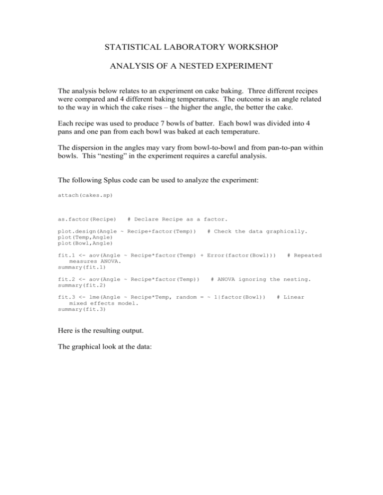
STATISTICAL LABORATORY WORKSHOP
ANALYSIS OF A NESTED EXPERIMENT
The analysis below relates to an experiment on cake baking. Three different recipes
were compared and 4 different baking temperatures. The outcome is an angle related
to the way in which the cake rises – the higher the angle, the better the cake.
Each recipe was used to produce 7 bowls of batter. Each bowl was divided into 4
pans and one pan from each bowl was baked at each temperature.
The dispersion in the angles may vary from bowl-to-bowl and from pan-to-pan within
bowls. This “nesting” in the experiment requires a careful analysis.
The following Splus code can be used to analyze the experiment:
attach(cakes.sp)
as.factor(Recipe)
# Declare Recipe as a factor.
plot.design(Angle ~ Recipe+factor(Temp))
plot(Temp,Angle)
plot(Bowl,Angle)
# Check the data graphically.
fit.1 <- aov(Angle ~ Recipe*factor(Temp) + Error(factor(Bowl)))
measures ANOVA.
summary(fit.1)
fit.2 <- aov(Angle ~ Recipe*factor(Temp))
summary(fit.2)
# ANOVA ignoring the nesting.
fit.3 <- lme(Angle ~ Recipe*Temp, random = ~ 1|factor(Bowl))
mixed effects model.
summary(fit.3)
Here is the resulting output.
The graphical look at the data:
# Repeated
# Linear
36
205
35
195
34
2
33
mean of Angle
3
1
32
185
175
Recipe1
factor(Temp)
35
20
25
30
Angle
40
45
50
Factors
175
180
185
190
195
200
205
35
30
25
20
Angle
40
45
50
Temp
5
10
15
Bowl
20
The repeated measures ANOVA:
summary(fit.1)
Error: factor(Bowl)
Df Sum of Sq Mean Sq
F Value
Pr(F)
Recipe1 2
40.500 20.2500 0.08657663 0.9174448
Residuals 18 4210.143 233.8968
Error: Within
Df Sum of Sq Mean Sq F Value
Pr(F)
factor(Temp) 3
306.952 102.3175 4.594986 0.0061659
Recipe1:factor(Temp) 6
77.119 12.8532 0.577225 0.7467591
Residuals 54 1202.429 22.2672
ANOVA ignoring the nesting:
> fit.2 <- aov(Angle ~ Recipe1 * factor(Temp))
> # ANOVA ignoring the nesting.
summary(fit.2)
Df Sum of Sq Mean Sq F Value
Pr(F)
Recipe1 2
40.500 20.2500 0.269373 0.7646248
factor(Temp) 3
306.952 102.3175 1.361064 0.2615823
Recipe1:factor(Temp) 6
77.119 12.8532 0.170978 0.9837826
Residuals 72 5412.571 75.1746
Note that the residual sum of squares combines the separate residual sums of squares
in the original analysis. The large bowl-to-bowl variation gives a much higher
residual mean square for the temperature effect, which now fails to reach
statistical significance.
The linear mixed effects model, which includes a random effect for bowls, but uses a
linear regression model for the temperature effect rather than an ANOVA model.
> fit.3 <- lme(Angle ~ Recipe1 * Temp, random =
> # Linear mixed effects model.
summary(fit.3)
Linear mixed-effects model fit by REML
Data: NULL
AIC
BIC
logLik
560.55 579.4037 -272.275
~ 1 | factor(Bowl))
Random effects:
Formula: ~ 1 | factor(Bowl)
(Intercept) Residual
StdDev:
7.291322 4.609049
Fixed effects: Angle ~ Recipe1 *
Value Std.Error
(Intercept)
2.59048
8.70753
Recipe11 -11.02857 10.66450
Recipe12
2.85476
6.15715
Temp
0.16381
0.04498
Recipe11Temp
0.06143
0.05509
Recipe12Temp -0.01333
0.03181
Temp
DF
t-value p-value
60 0.297498 0.7671
18 -1.034138 0.3148
18 0.463650 0.6485
60 3.641853 0.0006
60 1.115085 0.2693
60 -0.419215 0.6766
Standardized Within-Group Residuals:
Min
Q1
Med
Q3
Max
-2.019586 -0.6278114 -0.04249586 0.5601622 2.36891
Number of Observations: 84
Number of Groups: 21
Below are code and output from an analysis in SPSS. The default analysis in SPSS
breaks down the sum of squares due to the “within bowls” factor using a set of
orthogonal contrasts. I chose to use polynomial contrasts (the default), so that the
temperature effect is decomposed into linear, quadratic and cubic components.
To analyze these data in SPSS, each line in the file must give the data for 1 bowl and
the 4 results for each bowl need to be entered as distinct variables. These
variables are called Angle1, …, Angle4 in my data file. The command
WSFACTOR declares that these four outcomes differ because of “temp”.
Here is the code:
GLM
Angle1 Angle2 Angle3 Angle4 BY Recipe
/WSFACTOR = temp 4 Polynomial
/METHOD = SSTYPE(3)
/CRITERIA = ALPHA(.05)
/WSDESIGN = temp
/DESIGN = Recipe .
Here is some of the output:
Te sts of W ithi n-Subje cts Effects
Measure: MEA SURE_1
Source
temp
temp * Rec ipe
Error(t emp)
Sphericity Ass umed
Greenhous e-Geiss er
Huynh-Feldt
Lower-bound
Sphericity Ass umed
Greenhous e-Geiss er
Huynh-Feldt
Lower-bound
Sphericity Ass umed
Greenhous e-Geiss er
Huynh-Feldt
Lower-bound
Ty pe III Sum
of Squares
306.952
306.952
306.952
306.952
77.119
77.119
77.119
77.119
1202.429
1202.429
1202.429
1202.429
df
3
2.252
2.876
1.000
6
4.503
5.751
2.000
54
40.530
51.760
18.000
Mean Square
102.317
136.323
106.746
306.952
12.853
17.125
13.410
38.560
22.267
29.668
23.231
66.802
F
4.595
4.595
4.595
4.595
.577
.577
.577
.577
Sig.
.006
.013
.007
.046
.747
.700
.740
.572
Tests of Within-Subjects Contrasts
Measure: MEASURE_1
Source
temp
temp * Recipe
Error(temp)
temp
Linear
Quadratic
Cubic
Linear
Quadratic
Cubic
Linear
Quadratic
Cubic
Type III Sum
of Squares
281.752
.429
24.771
30.148
39.071
7.900
365.800
619.000
217.629
df
1
1
1
2
2
2
18
18
18
Mean Square
281.752
.429
24.771
15.074
19.536
3.950
20.322
34.389
12.090
F
13.864
.012
2.049
.742
.568
.327
Tests of Between-Subjects Effects
Measure: MEASURE_1
Transformed Variable: Average
Source
Intercept
Recipe
Error
Type III Sum
of Squares
95478.857
40.500
4210.143
df
1
2
18
Mean Square
95478.857
20.250
233.897
F
408.209
.087
Sig.
.000
.917
Sig.
.002
.912
.169
.490
.576
.725