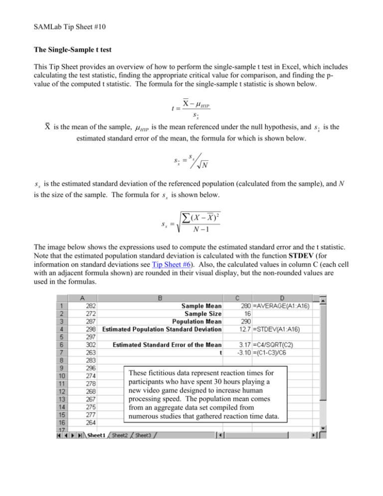
SAMLab Tip Sheet #10
The Single-Sample t test
This Tip Sheet provides an overview of how to perform the single-sample t test in Excel, which includes
calculating the test statistic, finding the appropriate critical value for comparison, and finding the pvalue of the computed t statistic. The formula for the single-sample t statistic is shown below.
t
X   HYP
sx
X is the mean of the sample,  HYP is the mean referenced under the null hypothesis, and s x is the
estimated standard error of the mean, the formula for which is shown below.
sx 
sx
N
s x is the estimated standard deviation of the referenced population (calculated from the sample), and N
is the size of the sample. The formula for s x is shown below.
sx 
(X  X )
2
N 1
The image below shows the expressions used to compute the estimated standard error and the t statistic.
Note that the estimated population standard deviation is calculated with the function STDEV (for
information on standard deviations see Tip Sheet #6). Also, the calculated values in column C (each cell
with an adjacent formula shown) are rounded in their visual display, but the non-rounded values are
used in the formulas.
These fictitious data represent reaction times for
participants who have spent 30 hours playing a
new video game designed to increase human
processing speed. The population mean comes
from an aggregate data set compiled from
numerous studies that gathered reaction time data.
SAMLab Tip Sheet #10
Our next step is to find the critical value with which to compare our computed t statistic. First, click in a
cell near your computed t statistic and select “Function” from the Insert menu (below left). Next select
“Statistical” from the Function category list and then select “TINV” from the Function name list (below
right). Click OK.
When you see the dialogue box below, input your alpha level (we will use 0.05) into the “Probability”
field and degrees of freedom in the “Deg_freedom” field. The degrees of freedom value for a singlesample t test is N – 1, where N is the size of the sample. Notice that Excel automatically assumes we
want the two-tailed critical value. You can check to see that the critical value Excel returns is correct
with a table in a statistics textbook. Click OK when you have entered the values.
Your output should resemble the image below. Note that Excel returns a positive critical value. This is
not a problem because we know that the negative critical value has the same magnitude because
Student’s t distribution is symmetrical.
SAMLab Tip Sheet #10
From our critical value we can see that we should reject our null hypothesis. However, it is also useful
to know the two-tailed p-value associated with our computed t statistic. Following the steps for
inserting TINV above, select a nearby cell and insert TDIST. You should see the dialogue box below.
For “X,” enter the absolute value of your computed t statistic (Excel will not handle a negative value),
and input the degrees of freedom into the “Deg_freedom” field as done previously. In the “Tails” field,
enter the number 2. When you have entered these values click OK.
Your worksheet should now resemble the one below. What do you conclude? Does the video game
work or should the researcher look elsewhere for trying to improve processing speed? Do not forget that
decreased reaction times denote increased processing speed!