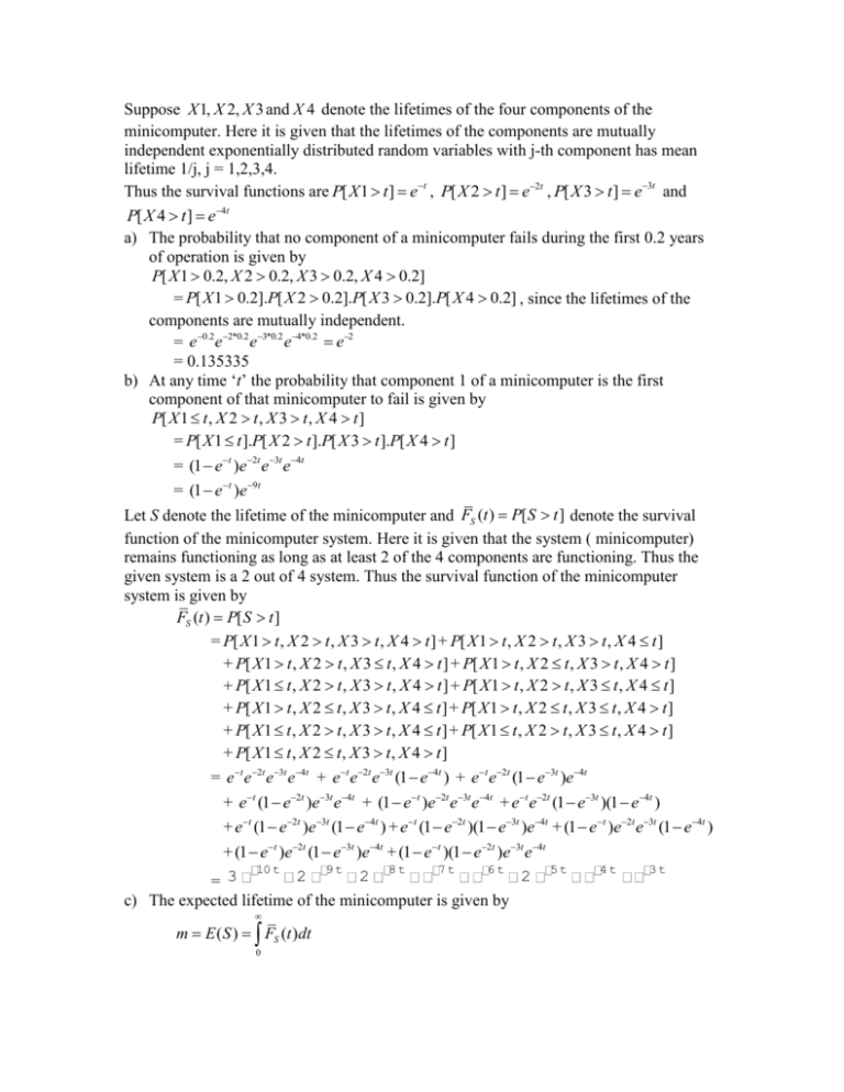
Suppose X 1, X 2, X 3 and X 4 denote the lifetimes of the four components of the
minicomputer. Here it is given that the lifetimes of the components are mutually
independent exponentially distributed random variables with j-th component has mean
lifetime 1/j, j = 1,2,3,4.
Thus the survival functions are P[ X 1  t ]  et , P[ X 2  t ]  e2t , P[ X 3  t ]  e3t and
P[ X 4  t ]  e4t
a) The probability that no component of a minicomputer fails during the first 0.2 years
of operation is given by
P[ X 1  0.2, X 2  0.2, X 3  0.2, X 4  0.2]
= P[ X 1  0.2].P[ X 2  0.2].P[ X 3  0.2].P[ X 4  0.2] , since the lifetimes of the
components are mutually independent.
= e0.2 e2*0.2 e3*0.2 e4*0.2  e2
= 0.135335
b) At any time ‘t’ the probability that component 1 of a minicomputer is the first
component of that minicomputer to fail is given by
P[ X 1  t , X 2  t , X 3  t , X 4  t ]
= P[ X 1  t ].P[ X 2  t ].P[ X 3  t ].P[ X 4  t ]
= (1  et )e2t e3t e4t
= (1  et )e9t
Let S denote the lifetime of the minicomputer and FS (t )  P[ S  t ] denote the survival
function of the minicomputer system. Here it is given that the system ( minicomputer)
remains functioning as long as at least 2 of the 4 components are functioning. Thus the
given system is a 2 out of 4 system. Thus the survival function of the minicomputer
system is given by
FS (t )  P[ S  t ]
= P[ X 1  t , X 2  t , X 3  t , X 4  t ] + P[ X 1  t , X 2  t , X 3  t , X 4  t ]
+ P[ X 1  t , X 2  t , X 3  t , X 4  t ] + P[ X 1  t , X 2  t , X 3  t , X 4  t ]
+ P[ X 1  t , X 2  t , X 3  t , X 4  t ] + P[ X 1  t , X 2  t , X 3  t , X 4  t ]
+ P[ X 1  t , X 2  t , X 3  t , X 4  t ] + P[ X 1  t , X 2  t , X 3  t , X 4  t ]
+ P[ X 1  t , X 2  t , X 3  t , X 4  t ] + P[ X 1  t , X 2  t , X 3  t , X 4  t ]
+ P[ X 1  t , X 2  t , X 3  t , X 4  t ]
= et e2t e3t e4t + et e2t e3t (1  e4t ) + et e2t (1  e3t )e4t
+ et (1  e2t )e3t e4t + (1  et )e2t e3t e4t + et e2t (1  e3t )(1  e4t )
+ et (1  e2t )e3t (1  e4t ) + et (1  e2t )(1  e3t )e4t + (1  et )e2t e3t (1  e4t )
+ (1  et )e2t (1  e3t )e4t + (1  et )(1  e2t )e3t e4t
10 t
7t
6t
4t
3t
2 9t 2 8t
2 5t
= 3
c) The expected lifetime of the minicomputer is given by

m  E ( S )   FS (t )dt
0
10 t
3
=
2
9t
2
8t
7t
6t
2
5t
4t
3t
t
0
3 2 2 1 1 2 1 1 158
       =
10 9 8 7 6 5 4 3 315
= 0.501587 = (1/2) years approximately
d) The variance of the lifetime of the minicomputer is given by
=

  Var ( S )  2 tFS (t )dt  m 2 ( This is the standard formula for variance for
2
0
positive random variables)

But 2  tFS (t )dt =
2
t
10 t
3
2
9t
2
8t
7t
6t
2
5t
4t
3t
t
0
0
=
569897
= 0.358968
1587600
2
569897  158 
170473

 
1587600  315  1587600
= 0.107378
e) Let N(t) denote the number of renewal in the interval [0, t]. Then { N(t), t ≥ 0} will
be a Poisson process if the interarrival times ( the time between successive
replacement of the minicomputer ), the random variable S must be exponentially
distributed. That is the survival function of S must be of the form
FS (t )  P[ S  t ]  e  t . But here the distribution of S is not exponentially distributed
as its survival function is of the form
10 t
7t
6t
4t
3t
2 9t 2 8t
2 5t
F (t )  3
, which is
Thus  2 =
S
not the survival function of an Exponential random variable. Thus { N(t), t ≥ 0} is not
a Poisson process.
f) Even though { N(t), t ≥ 0} is not a Poisson process, it is a renewal process since the
interarrival times are identically distributed with the survival function FS (t ) .
By the theory of renewal process for sufficiently large ‘t’
 n  (t / m) 
P[ N (t )  n]   
 , where  (.) is the cumulative distribution function
3
  t/m 
of a Standard Normal random variable ( For the Proof refer Ross( 1996, page 109)
Ross, S.M Stochastic Processes, 2nd Ed. Wiley, New York )
Now the probability that at least 50 computers have to be replaced during the first 10
years of operation of the alarm system is given by
 50  (10 / m) 
P[ N (10)  50]  1  P[ N (10)  50]  1   

3
  10 / m 
where m = 0.501587 and  =  2  0.327686
Substituting these values we get
P[ N (10)  50]  1   10.3062  =1-1 = 0