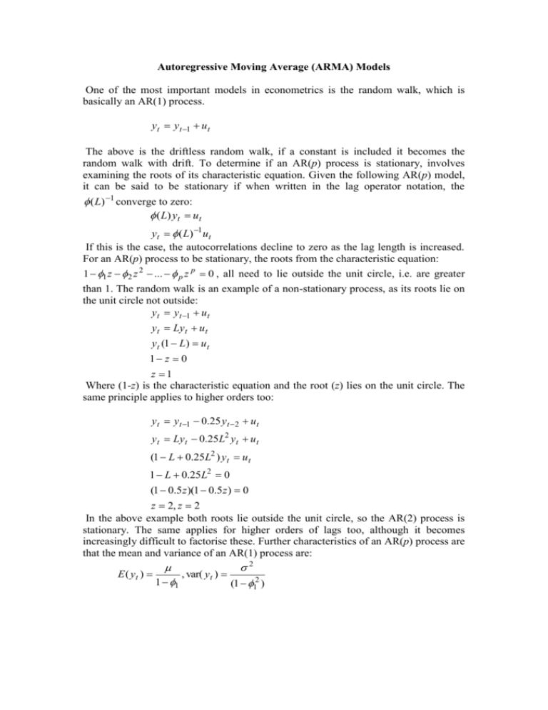
Autoregressive Moving Average (ARMA) Models
One of the most important models in econometrics is the random walk, which is
basically an AR(1) process.
yt  yt 1  ut
The above is the driftless random walk, if a constant is included it becomes the
random walk with drift. To determine if an AR(p) process is stationary, involves
examining the roots of its characteristic equation. Given the following AR(p) model,
it can be said to be stationary if when written in the lag operator notation, the
 ( L) 1 converge to zero:
 ( L) y t  u t
yt   ( L) 1 ut
If this is the case, the autocorrelations decline to zero as the lag length is increased.
For an AR(p) process to be stationary, the roots from the characteristic equation:
1  1 z   2 z 2  ...   p z p  0 , all need to lie outside the unit circle, i.e. are greater
than 1. The random walk is an example of a non-stationary process, as its roots lie on
the unit circle not outside:
yt  yt 1  u t
yt  Lyt  u t
yt (1  L)  u t
1 z  0
z 1
Where (1-z) is the characteristic equation and the root (z) lies on the unit circle. The
same principle applies to higher orders too:
yt  yt 1  0.25 yt 2  u t
yt  Lyt  0.25L2 yt  u t
(1  L  0.25L2 ) yt  u t
1  L  0.25L2  0
(1  0.5 z )(1  0.5 z )  0
z  2, z  2
In the above example both roots lie outside the unit circle, so the AR(2) process is
stationary. The same applies for higher orders of lags too, although it becomes
increasingly difficult to factorise these. Further characteristics of an AR(p) process are
that the mean and variance of an AR(1) process are:

2
E ( yt ) 
, var( yt ) 
1  1
(1  12 )
Box-Jenkins Methodology
This is the technique for determining the most appropriate ARMA or ARIMA model
for a given variable. It comprises four stages in all:
1) Identification of the model, this involves selecting the most appropriate
lags for the AR and MA parts, as well as determining if the variable
requires first-differencing to induce stationarity. The ACF and PACF are
used to identify the best model. (Information criteria can also be used)
2) Estimation, this usually involves the use of a least squares estimation
process.
3) Diagnostic testing, which usually is the test for autocorrelation. If this part
is failed then the process returns to the identification section and begins
again, usually by the addition of extra variables.
4) Forecasting, the ARIMA models are particularly useful for forecasting due
to the use of lagged variables.
The Box-Jenkins methodology is often referred to as more an art then a science, this
lack of theory behind the models is one criticism of them, however they are used as an
effective model for forecasting.
Forecasting
One of the most important tests of any model is how well it forecasts. This can
involve either in-sample or out-of-sample forecasts, usually the out-of-sample
forecasts are viewed as the most informative, as the data used for the forecast is not
included in the estimation of the model used for the forecast. When assessing how
well a model forecasts, we need to compare it to the actual data, this then produces a
forecast vale, an actual value and a forecast error (difference between forecast and
actual values) for each individual observation used for the forecast. Then the accuracy
of the forecast needs to be measured, this can be done by:
1) Plot of forecast values against actual values
2) Use of a statistic such as the Mean Square Error (MSE) or RMSE
(R stands for Root).
3) Use of Theil’s U coefficient, which in effect compares the forecast
to a benchmark forecast.
4) The use of financial loss functions, where the % of correct sign
predictions or direction change predictions are calculated. This is
particularly important in fiancé, as if you can forecast the sign
correctly, it usually means a profit can be made.
When forecasting future values of a variable, it is often important to have a
benchmark model, such as the random walk to compare the forecasts of the model
with, if it can not beat the random walk it can be argued to be a relatively poor
forecaster, the random walk often wins!