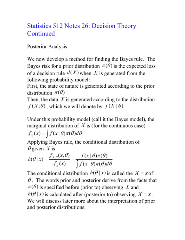
Statistics 512 Notes 26: Decision Theory
Continued
Posterior Analysis
We now develop a method for finding the Bayes rule. The
Bayes risk for a prior distribution  ( ) is the expected loss
of a decision rule d ( X ) when X is generated from the
following probability model:
First, the state of nature is generated according to the prior
distribution  ( )
Then, the data X is generated according to the distribution
f ( X ; ) , which we will denote by f ( X |  )
Under this probability model (call it the Bayes model), the
marginal distribution of X is (for the continuous case)
f X ( x)   f ( x |  ) ( )d
Applying Bayes rule, the conditional distribution of
 given X is
f ( x,  )
f ( x |  ) ( )
h( | x)  X ,

f X ( x)
 f ( x |  ) ( )d
The conditional distribution h( | x ) is called the X  x of
 . The words prior and posterior derive from the facts that
 ( ) is specified before (prior to) observing X and
h( | x ) is calculated after (posterior to) observing X  x .
We will discuss later more about the interpretation of prior
and posterior distributions.
Suppose that we have observed X  x . We define the
posterior risk of an action a  d ( x ) as the expected loss,
where the expectation is taken with respect to the posterior
distribution of  . For continuous random variables, we
have
Eh ( | X  x ) [l ( ), d ( x))]   l ( , d ( x))h( | X  x)d
Theorem: Suppose there is a function d0 ( x) that minimizes
the posterior risk. Then d0 ( x) is a Bayes rule.
Proof: We will this for the continuous case. The discrete
case is proved analogously. The Bayes risk of a decision
function d is
B(d )  E ( ) [ R( ), d ]
 E ( ) [ E X (l ( , d ( X )) |  ]
    l ( , d ( x)) f ( x |  ) dx  ( ) d


  l ( , d ( x)) f x , ( x,  ) dxd
    l ( , d ( x)) h( | x) d  f X ( x) dx


(We have used the relations
f ( x |  ) ( )  f X , ( x,  )  f X ( x)h( | x) )
Now the inner integral is the posterior risk and since
f X ( x) is nonnegative, B(d ) can be minimized by choosing
d ( x)  d 0 ( x) .

The practical importance of this theorem is that it allows us
to use just the observed data, x , rather than considering all
possible values of X to find the action for the Bayes rule
d ** given the data X  x , d ** ( x) . In summary the
**
algorithm for finding d ( x) is as follows:
Step 1: Calculate the posterior distribution h( | X  x) .
Step 2: For each action a , calculate the posterior risk,
which is
E[l ( , a) | X  x]   l ( , a)h( | X )d
*
The action a that minimizes the posterior risk is the Bayes
**
*
rule action d ( x)  a
Example: Consider again the engineering example.
Suppose that we observe X  x2  45 . In the notation of
that example, the prior distribution is  (1 )  .8 ,  (2 )  .2 .
We first calculate the posterior distribution:
f ( x |  ) (1 )
h(1 | x2 )  2 2 1
 i 1 f ( x2 | i ) (i )
.3*.8
.3*.8  .2*.2
 .86

Hence,
h(2 | x2 )  .14
We next calculate the posterior risk (PR) for a1 and a2 :
PR(a1 )  l (1 , a1 )h(1 | x2 )  l ( 2 , a1 )h( 2 | x2 )
 0  400*.14
 56
and
PR(a2 )  l (1 , a2 )h(1 | x2 )  l ( 2 , a2 )h( 2 | x2 )
 100*.86  0
 86
Comparing the two, we see that a1 has the smaller posterior
risk and is thus the Bayes rule.
Decision Theory for Point Estimation
Estimation theory can be cast in a decision theoretic
framework. The action space is the same as the parameter
space and the decision functions are point estimates
d ( X )  ˆ . In this framework, a loss function may be
specified, and one of the strengths of the theory is that
general loss functions are allowed and thus the purpose of
estimation is made explicit. But the case of squared error
loss is especially tractable. For squared error loss, the risk
is

R( , d )  E   d ( X 1 ,

, X n )
2


2

ˆ
 E    


Suppose that a Bayesian approach is taken and the prior
distribution on  is  ( ) . Then from the above theorem,
the Bayes rule for squared error loss can be found by
minimizing the posterior risk, which is
E ( ) [(  ˆ)2 | X  x] . We have
E ( ) [(  ˆ)2 | X  x]  Var ( ) (  ˆ) | X  x    E ( ) (  ˆ) | X  x 
 Var ( )  | X  x    E ( )  | X  x   ˆ 
2
The first term of this last expression does not depend on ˆ
ˆ
ˆ
and the second term is minimized by   E ( )  | X  x  .
Thus, the Bayes rule for squared error loss is the mean of
the posterior distribution of  ,
ˆ    h( | X )d .
Example: A (possibly) biased coin is thrown once, and we
want to estimate the probability of the coin landing heads
on future tosses based on this single toss. Suppose that we
have no idea how biased the coin is; to reflect this state of
knowledge, we use a uniform prior distribution on  :
g ( )  1, 0    1
Let X  1 if a head appears, and let X  0 if a tail appears.
The distribution of X given  is
x 1
 ,
f (x |  )  
1   , x  0
The posterior distribution is
f ( x |  ) 1
h( | x) 
 f ( x |  )d
In particular,
2
h( | X  1) 

1
 2
  d
0
h( | X  0) 
(1   ) 1
1
 2(1   )
 (1   )d
0
Suppose that X  1 . The Bayes estimate of  is the mean
of the posterior distribution h( | X  1) , which is
1
2

(2

)
d


0
3
ˆ1

The Bayes estimate in the case where X  0 is
3.
Note that these estimates differ from the classical
maximum likelihood estimates, which are 0 and 1.
Comparison of the risk functions of the Bayes estimate and
the MLE:
The risk function of the above Bayes estimate is


2
2
2
1

2

E  ˆBayes         P ( X  0)      P ( X  1)

  3

3

2
2
1

2

     (1   )      
3

3

1 1
1
    2
9 3
3
The risk function of the MLE ˆMLE  X is


2
2
2
E  ˆMLE      0    P ( X  0)  1    P ( X  1)


  0    (1   )  1    
2
2
  2     (1   )
The following graph shows the risk function of the Bayes
estimate and the MLE – the Bayes estimate is the solid line
and the MLE is the dashed line. The Bayes estimate has
smaller risk than that of the MLE over most of the range of
[0,1] but neither estimator dominates the other.
Admissibility
Minimax estimators and Bayes estimators are “good
estimators” in the sense that their risk functions have
certain good properties; minimax estimators minimize the
worst case risk and Bayes estimators minimize a weighted
average of the risk. It is also useful to characterize bad
estimators.
Definition: An estimator ˆ is inadmissible if there exists
another estimator ˆ ' that dominates ˆ , meaning that
R( ,ˆ ')  R( , ˆ) for all  and
R( ,ˆ ')  R( , ˆ) for at least one 
If there is no estimator ˆ' that dominates ˆ, then ˆ is admissible
Example: Let X be a sample of size one from a
N ( ,1) distribution and consider estimating  with squared
error loss.
Let ˆ( X )  2 X . Then
R( ,ˆ)  E [(2 X   ) 2 ]

 Var (2 X )   E [2 X ]   
2
 4  2
The risk function of the MLE ˆMLE ( X )  X is
R( ,ˆMLE )  E [( X   ) 2 ]
 Var ( X )   E [ X ]   
2
1
Thus, the MLE dominates ˆ( X )  2 X and ˆ( X )  2 X is
inadmissible.
Consider another estimator ˆ( X )  3 . We will show that
ˆ is admissible. Suppose not. Then there exists a different
estimator ˆ ' with smaller risk. In particular,
R(3, ˆ ')  R(3, ˆ)  0 . Hence,
0  R(3, ˆ ')   (ˆ ' 3) 2


1
exp ( x  3) 2 / 2 dx .
2
Thus, ˆ '( X )  3 and there is no estimator that dominates
ˆ . Even though ˆ is admissible, it is clearly a bad
estimator.
In general, it is very hard to know whether a particular
estimate is admissible, since one would have to check that
it was not strictly dominated by any other estimate in order
to show that it was admissible. The following theorem
states that any Bayes estimate is admissible.
Theorem (Complete Class Theorem): Suppose that one of
the following two assumptions holds:
(1)  is discrete and d * is a Bayes rule with respect to a
prior probability mass function  such that  ( )  0 for all
  .
(2)  is an interval and d * is a Bayes rule with respect to a
prior density function g ( ) such that  ( )  0 for all
  and R ( , d ) is a continuous function of  for all d .
Then d * is admissible.
Proof: We will prove the theorem for assumption (2). The
proof is by contradiction. Suppose that d * is inadmissible.
There is then another estimate, d , such that
R( , d *)  R( , d ) for all  and with strict inequality for
some  , say 0 . Since R( , d *)  R( , d ) is a continuous
function of  , there is an   0 and an interval   h such
that
R( , d *)  R( , d )   for 0  h    0  h
Then,
0  h

  R( , d *)  R( , d ) ( )d     R( , d *)  R( , d ) ( )d

0 h

0  h


 ( )d  0
0 h
But this contradicts the fact that d * is a Bayes rule because
a Bayes rule has the property that

B(d *)  B(d ) 
  R( , d *)  R( , d ) ( )d  0 .

The proof is complete.

The theorem can be regarded as both a positive and
negative result. It is positive in that it identifies a certain
class of estimates as being admissible, in particular, any
Bayes estimate. It is negative in that there are apparently
so many admissible estimates – one for every prior
distribution that satisfies the hypotheses of the theorem –
and some of these might make little sense (like ˆ( X )  3
for the normal distribution above).