Master AWT, 1st year, 2014-2015, 1st semester
Author: Ș.L. Dr. ing. Octaviana Datcu
1
Laboratory 1
Random processes
Purpose: lead to assimilation of the notions students learned during the lecture. Symbolic
and numeric solving specific problems arising in signal processing random, and the calculation and
representation of the autocorrelation function and power spectral density is combined with the use of
MATLAB programming language as a means of verification.
Students will:
1. read and understand Applications 1, 2 and 3;
2. solve Exercises 1-3 during the laboratory session, following the schema given as example when
solving the applications. They will give to the instructor, at the end of the lab session, the solved
exercises, in „Name1Name2.doc” format.
3. solve Homework 1-9 in 2 weeks. At the 2nd lab session, they will bring, in electronic format, the
exercises solved in the same manner the ones during the lab 1 were solved.
Application 1
1.5
be. a)
z  2.5  z 1
Graphically represent Pxx (e j ),   ( ,  ]; b) Compute the autocorrelation function; c) Graphically
represent the autocorrelation function; d) Compute the average power of the process.
Let a random process with zero average and power spectral density Pxx ( z ) 
Solution
a) Pxx (e j ) 
e
j
1.5
1.5

,   ( ,  ]
 j
2.5  2 cos 
 2.5  e
e j  cos   j sin 
e  j  cos   j sin 
-------------------------e j  e  j  2 cos 
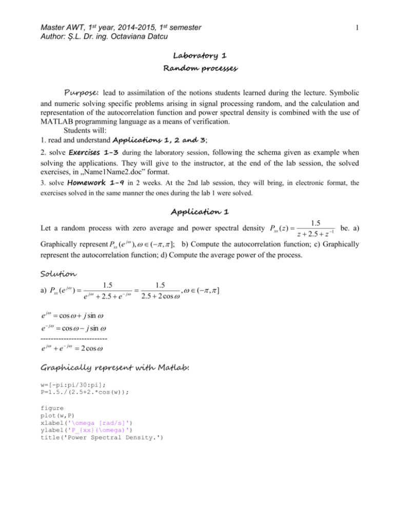
Graphically represent with Matlab:
w=[-pi:pi/30:pi];
P=1.5./(2.5+2.*cos(w));
figure
plot(w,P)
xlabel('\omega [rad/s]')
ylabel('P_{xx}(\omega)')
title('Power Spectral Density.')
Master AWT, 1st year, 2014-2015, 1st semester
Author: Ș.L. Dr. ing. Octaviana Datcu
b) Pxx ( z ) 
1.5
1
1


1
1
z  2.5  z
1  0.5  z
1  2  z 1
 the autocorrelation function is given by:
1
1


rxx (n)  c xx (n)  Z 1{Pxx ( z )}  Z 1 

 a |n| , a  0.5.
1
1 
1 2  z 
1  0.5  z
1.5
1
1


1
1
z  2.5  z
1  0.5  z
1  2  z 1
0, n  0
It is known that u (n)  
is the Heaviside step function.
1, n  0
c) Graphically represent the autocorrelation function with Matlab:
a=-0.5;
n=[-20:1:20]
r=a.^abs(n);
figure
plot(n,r)
xlabel('n')
ylabel('r_{xx}(n)')
title('Autocorrelation function.')
2
Master AWT, 1st year, 2014-2015, 1st semester
Author: Ș.L. Dr. ing. Octaviana Datcu
3
d) The average power is given by the value of the autocorrelation function in its origin.
 rxx (0)  (0.5)|n|
n 0
 (0.5)|0|  1W
Exercise 1
40 z
be. a)
 99 z  202 z  99
Graphically represent Pxx (e j ),   ( ,  ]; b) Compute the autocorrelation function; c) Graphically
represent the autocorrelation function; d) Compute the average power of the process.
Let a random process with zero average and power spectral density Pxx ( z ) 
2
Exercițiul 2
10
. be. a)
5  4 cos 2
Graphically represent Pxx (e j ),   ( ,  ]; b) Compute the autocorrelation function; c) Graphically
represent the autocorrelation function; d) Compute the average power of the process.
Let a random process with zero average and power spectral density Pxx (e j ) 
Temă
1.2 cos   2
be.
1.2 cos   1.36
a) Graphically represent Pxx (e j ),   ( ,  ];
b) Compute the autocorrelation function; c)
Graphically represent the autocorrelation function; d) Compute the average power of the process.
1. Let a random process with zero average and power spectral density Pxx (e j ) 
4
Master AWT, 1st year, 2014-2015, 1st semester
Author: Ș.L. Dr. ing. Octaviana Datcu
2. Let the wide sense stationary random process with the power spectral density given by
( z  1) 2
be. a) Graphically represent Pxx (e j ),   ( ,  ]; b) Compute the autocorrelation
z
function; c) Graphically represent the autocorrelation function; d) Compute the average power of the
process.
3. Let the wide sense stationary random process with the power spectral density given by
Pxx ( z ) 
( z  1) 2
be. a) Graphically represent Pxx (e j ),   ( ,  ]; b) Compute the autocorrelation
z
function; c) Graphically represent the autocorrelation function; d) Compute the average power of the
process.
4. Let the wide sense stationary random process with the power spectral density given by
z
Pxx ( z )  2
, | a | 1, be. a) Graphically represent Pxx (e j ),   ( ,  ], for a  0.1 and
az  (1  a 2 ) z  a
a  0.9. b) Compute the autocorrelation function; c) Graphically represent the autocorrelation
function; d) Compute the average power of the process. e) Represent Pxx (e j ),   ( ,  ], for | a | 1,
with a 0.1 step.
5. Let the wide sense stationary random process with the power spectral density given by
z
Pxx ( z ) 
, | a | 1, be. a) Graphically represent Pxx (e j ),   ( ,  ], for a  0.1 and
( z  a)(1  az )
a  0.9. b) Compute the autocorrelation function; c) Graphically represent the autocorrelation
function; d) Compute the average power of the process. e) Represent Pxx (e j ),   ( ,  ], for | a | 1,
with a 0.1 step.
Pxx ( z ) 
Application 2
A causal linear time invariant system is described by y (n)  0.6 y (n  1)  x(n)  1.25 x(n  1). Its input
1
. a) Compute the power spectral density of its output; b) Represent, on
has Pxx (e j ) 
1.64  1.6 cos 
the same figure, the power spectral densities for its input, and for its output respectively, for
  ( ,  ]. .
Solution
a)


1  1.25 z 1
1  1.25e  j
j
 H (e ) 
.
The transfer function of the system is H ( z ) 
1  0.6 z 1
1  0.6e  j
The power spectral density at the output of the system is:
Master AWT, 1st year, 2014-2015, 1st semester
Author: Ș.L. Dr. ing. Octaviana Datcu
1
1  1.25e  j
Pyy (e )  Pxx (e ) | H (e ) | 

1.64  1.6 cos  1  0.6e  j
j
j
 Pyy (e j ) 
1  1.25e  j
1  0.6e  j
2
j
2
5
2

1
1  2.5 cos   1.5625
2.5 cos   2.56


1.64  1.6 cos  1  1.2 cos   0.36
2.23  0.21cos   1.92 cos 2 
2
 1  2.5 cos   1.5625 cos 2   1.5625 sin 2 
1  1.25(cos   j sin  )



1  0.6(cos   j sin  )
1  1.2 cos   0.36 cos 2   0.36 sin 2 

1  1.25e  j

1  0.6e  j
2




2
2
 1  2.5 cos   1.5625 
1  2.5 cos   1.5625
 
 

1  1.2 cos   0.36
 1  1.2 cos   0.36 
b) The graphical representation:
Matlab code:
w=[-pi:pi/30:pi];
Px=1./(1.64+1.6.*cos(w));
figure
plot(w,Px)
xlabel('\omega [rad/s]')
ylabel('P_{xx}(\omega) [W/Hz]')
title('Power spectral density.')
hold on
y=(2.5*cos(w)+2.56)./(2.23+0.21*cos(w)-1.92*cos(w).^2);
plot(w,Py,'r--')
The legend may be included manually (InsertLegendP_{xx}(\omega), P_{yy}(\omega)) or by
consulting help legend, from the Matlab command window.
Master AWT, 1st year, 2014-2015, 1st semester
Author: Ș.L. Dr. ing. Octaviana Datcu
6
Exercise 3
A white noise x(n) with the average power  2 is applied at the input of a filter with the transfer
function H ( z )  1  z 1 . Let y (n) be the output of the system. Compute the functions
rxy (n), ryx (n), ryy (n), the power spectral density and the average power of the output. Graphically
represent H (e j ),   ( ,  ] and Pyy (e j ),   ( ,  ].
Temă
6. A white noise x(n) with the average power  2 is applied at the input of a filter with the transfer
function H ( z )  1  z 1 . Let y (n) be the output of the system. Compute the functions
rxy (n), ryx (n), ryy (n), the power spectral density and the average power of the output. Graphically
represent H (e j ),   ( ,  ] and Pyy (e j ),   ( ,  ].
7. A white noise x(n) with the average power  2 is applied at the input of a filter with the transfer
1
. Let y (n) be the output of the system. Compute the functions
function H ( z ) 
1  az 1
rxy (n), ryx (n), ryy (n), the power spectral density and the average power of the output. Graphically
represent H (e j ),   ( ,  ] and Pyy (e j ),   ( ,  ].
8. A white noise x(n) with the average power  2 is applied at the input of a filter with the transfer
1
. Let y (n) be the output of the system. Compute the functions
function H ( z ) 
1  az 1
rxy (n), ryx (n), ryy (n), the power spectral density and the average power of the output. Graphically
represent H (e j ),   ( ,  ] and Pyy (e j ),   ( ,  ].
Application 3
A random process with rxx (k )  0.5 is applied to a system characterized by h(n)   (n)   (n  1) .
a) Compute the power spectral density of the input; b) represent the power spectral density of the
input; Pxx (e j ),   ( ,  ] ; c) compute the power spectral density of the output; d) represent the
power spectral density of the output; e) compute the autocorrelation function of the output; f) represent
the autocorrelation function of the output; g) compute the average power of the output.
k
Solution
a) Pxx ( z )  Z {0.5 k  u (n)  0.5  k  u (n  1)} 
1
1

1
1  0.5  z
1  2  z 1
1
1
1  2  e  j  1  0.5e  j
 1.5


 j

 j
 j
 j
 j
 2 j
1  0.5  e
1 2 e
1  2  e  0.5  e  e
e  2  0.5  e  j
b)
 1.5
1.5
 Pxx (e j ) 

cos   j sin   2.5  cos   j sin  2.5  2 cos 
Pxx (e j ) 
Master AWT, 1st year, 2014-2015, 1st semester
Author: Ș.L. Dr. ing. Octaviana Datcu
Matlab code:
w=[-pi:pi/30:pi];
P=1.5./(2.5-2*cos(w));
figure
plot(w,P)
xlabel('\omega [rad/s]')
ylabel('P_{xx}(\omega) [W/Hz]')
title('Power Spectral Density')
c) Pyy ( z )  Pxx ( z ) H ( z ) H ( z 1 ) 
d) Pyy (e j ) 
e
j
 1.5
(1  z 1 )(1  z )
z  2.5  z 1
 1.5
 1.5
 3(1  cos  )
(1  e  j )(1  e j ) 
(2  2 cos  ) 
 j
2 cos   2.5
2 cos   2.5
 2.5  e
Matlab code:
w=[-pi:pi/30:pi]
P=3*(1+cos(w))./(-2.5+2*cos(w));
figure
plot(w,P)
xlabel('\omega [rad/s]')
ylabel('P_{xx}(\omega) [W/Hz]')
title('Power Spectral Density')
7
Master AWT, 1st year, 2014-2015, 1st semester
Author: Ș.L. Dr. ing. Octaviana Datcu
8
Temă
9. A random process with rxx (n)  0.5
is applied to a system characterized by
h(n)   (n)   (n  1) . a) Compute the power spectral density of the input; b) represent the power
spectral density of the input; Pxx (e j ),   ( ,  ] ; c) compute the power spectral density of the
output; d) represent the power spectral density of the output; e) compute the autocorrelation function
of the output; f) represent the autocorrelation function of the output; g) compute the average power of
the output.
n
The residue method
Compute the autocorrelation function rxx (n), for a random process with the power spectral density
1.5 z
given by Pxx ( z ) 
.
( z  0.5)( z  2)
Solution
rxx (n)  Z 1{Pxx ( z )} 
rez


1
1
1.5 z
1.5 z n
n 1
n 1


z
P
(
z
)
dz

z
dz


xx



2j | z|1
2j | z|1
( z  0.5)( z  2)
i z i , | z i | 1 ( z  0.5)( z  2) 
The only pole interior to the circle of unity radius (which is the integration domain), for n  0, is
z1  0.5, so:




1.5 z n
1.5 z n
n
rxx (n)  rez 
  lim ( z  0.5)
  (0.5) , n  0.
( z  0.5)( z  2) 
zi 0.5 
zi  0.5  ( z  0.5)( z  2) 
n
For n  0, rxx (n)  rxx (n)  (0.5) .
 rxx (n)  (0.5) |n| , ()n.
Master AWT, 1st year, 2014-2015, 1st semester
Author: Ș.L. Dr. ing. Octaviana Datcu
Annex
Table I. Z transform. [Sursă: http://en.wikipedia.org/wiki/Z-transform]
9
Master AWT, 1st year, 2014-2015, 1st semester
Author: Ș.L. Dr. ing. Octaviana Datcu
Annex
Table I. Z transform. [Sursă: http://en.wikipedia.org/wiki/Z-transform] (continued)
10