MUTIPLE REGRESSION MODELS
Need for Several Predictor Variables, for example:



Study of short children: peak plasma growth hormone level (Y), with 14
predictors including gender, age, and various body measurements. [observational
data]
Study of the toxic action of a certain chemical on silkworm larvae : the survival
time (Y) of the silkworm larvae, with two predictor (explanatory or independent)
variables, including dose of the chemical in an aqueous solution and weight of the
larvae. [experimental data]
 A number of key variables affect the response variable in
important and distinctive ways
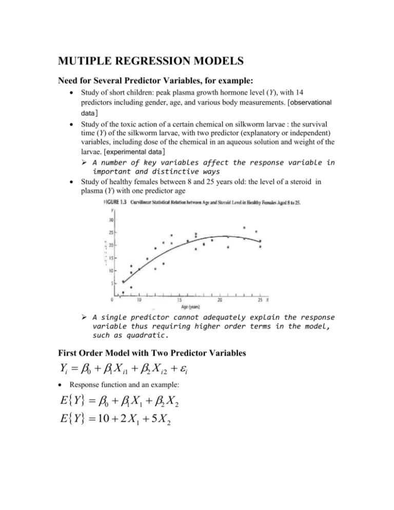
Study of healthy females between 8 and 25 years old: the level of a steroid in
plasma (Y) with one predictor age
 A single predictor cannot adequately explain the response
variable thus requiring higher order terms in the model,
such as quadratic.
First Order Model with Two Predictor Variables
Yi  0  1 X i1  2 X i 2  i

Response function and an example:
EY   0  1 X1  2 X 2
EY   10  2 X1  5 X 2
Meaning of Regression Coefficients
0  10 the intercept, mean response EY
only if X1  0,X 2  0 in range of mode
1  2  E{Y} when X1  1 and X 2 is held constant
 2  5  E{Y} when X 2  1 and X1 is held constant
1 ,  2 are called partial regression coefficients

In this example, when X1 changes, the change in Y is the same no matter what level X2
is held at, and vice versa. Such a model is called an additive effects model and the
predictors do not interact in the effects on Y.
First Order Model with More than Two Predictor Variables
Yi  0  1 X i1  2 X i 2  p 1 X i, p 1  i
General Linear Regression Model
Yi  0  1X i1   2 X i 2     p 1X i , p 1   i
0 , 1 ,...,  p 1 unknown parameters
X i1 ,..., X i , p 1 known constants

 i independen t N 0,  2

i=1,...,n

Response function
EY  0  1X1  2 X 2    p 1X p 1
p-1 Predictor Variables

When the predictor variables are all different, i.e. no variables are a combination of
any other variables, then the model is a first order model.
Qualitative Predictor Variables

Example: Predict length of hospital stay (Y) based on age (X1) and gender (X2) of the
patient.
Yi  0  1 X i1  2 X i 2  i
X i1  patient's age
1 if patient female
X i2 
0 if patient male

Response function
EY   0  1 X1  2 X 2
Male: X1  0
EY   0  1 X1
Female: X 2  1
EY   0  1  2 X 2
In general, represent a qualitative (categorical) variable with c classes by means of c-1
indicator variables. For example add disability status (not disabled, partially disables,
disabled) to hospital stay example:
Yi  0  1 X i1  2 X i 2  3 X i 3  4 X i 4  i
X
i1
 patient's age
1 if patient female

X

 i2

0
if
patient
male


1 if patient not disabled


X

 i 3 0 otherwise





1
if
patient
partially
disabled
X 

i4


0 otherwise


Polynomial Regression
Yi  0  1 X i  2 X i2  i
X i1  X i
X i 2  X i2

Response function is curvilinear
Transformed Variables
log Yi  0  1X i1   2 X i 2  3X i 3  i
Yi'  log Yi
Interaction Effects
Yi  0  1 X i1  2 X i 2  3 X i1 X i 2  i
X i 3  X i1 X i 2
Combination of Cases
Yi  0  1 X i1  2 X i21  3 X i 2  4 X i22  5 X i1 X i 2  i

In terms of the general linear regression model:
Zi1  X i1 Zi 2  X i21 Zi 3  X i 2 Zi 4  X i22 Zi 5  X i1 X i 2
Yi  0  1Zi1  2 Zi 2  3Zi 3  4 Zi 4  5 Zi 5  i
Meaning of “Linear” in General Linear Regression Model

The term linear model refers to the fact that the General Linear Regression Model is
linear in the parameters; it does not refer to the shape of the response surface.
Figure: Linear Models Typically Encountered in Empirical Studies
(1) Yi  0  1 X i1  2 X i 2
 i
(2) Yi  0  1 X i1  2 X i 2
 3 X i1 X i 2  i
(3) Yi  0  1X i1  2 X i 2
 3X i1X i 2
 4 X i21  5X i22
 i
( 4) Yi  0  1 X i1  2 X i 2
 3 X i1 X i 2  i
1 If class A
X i2 
0 If class B

Note: Model (1) is first order, Models (2) (4) are second order. The order of a model is
determined by the sum of exponents of the
variables in the most complex term.
GENERAL LINEAR REGRESSION MODEL IN
MATRIX TERMS

Algebraic form:
Y1  0  1 X11  2 X12  p 1 X1 p 1  1
Y2  0  1 X 21  2 X 22  p 1 X 2 p 1  2

Yn  0  1 X n1  1 X n 2  p 1 X np 1  n

Matrix entities:
 Y1 
Y 
2
Y 
n 1

 
Yn 
1 X11 X12  X1 p 1 

X 2 p 1 
1
X
X

21
22

X 
n p
  
 


X
1
X
X

np

1
n1
n2


 0 
  
1 
 
  
p 1



 p 1 
 1 
 
2
  
n 1

 
n 

Linear model in matrix terms:
Y X  
n 1
n  p p 1
n 1
  Normal
E  0
 2    2I
ESTIMATION OF REGRESSION COEFFICIENTS

The Method of Least Square
Q
n
 (Y  
i
0
 1X i1   2 X i 2     p 1X i ,p 1 ) 2
i 1

Normal Equations in matrix terms (derived by calculus):
X X b  X Y
p  p p 1

p 1
SS jj   X ij  X j

  X

2

Y  Y 
SS jk  SS kj   X ij  X j  X ik  X k 
SS jY  SS Yj
ij
 Xj
i
SS12  SS1, p 1 
 SS11
 SS
SS 22  SS 2, p 1 
21

X X  
p p
 





 SS p 1,1 SS p 1,2  SS p 1, p 1 
 SS1Y 
 SS 
2Y 
X Y  
p 1




SS
p

1
,
Y


Estimated Regression Coefficients
 X X 1 X Xb   X X 1 X Y
1
b   X X X Y
E b   , Unbiased


E b  E  X X X Y
1
  X X X E Y
1
  X X X X
1
 I  
FITTED VALUES AND RESIDUALS
Fitted Values
 Ŷ1 
 
Ŷ
Ŷ   2  Ŷ  X b  XXX 1 XY
   n1 np p1
n1
 
 Ŷn 

Hat Matrix
H  XXX 1 X
n n
Ŷ  H Y
n1
n n n1

Residuals
 e1 
e 
e   2  e  Y  Ŷ  Y  Xb
n1
   n1 n1 n1 n1 n1
 
e n 
e  Y  Ŷ  Y  HY  I  H Y

Variance-Covariance Matrix of Residuals
 2 e   2  I  H 
n n
s 2 e  MSE I  H
n n

Derivation of the variance-covariance matrix
 2  e   I  H   2  Y  I  H 

  I  H   2  e  I  H 
  2  I  H  I I  H 
  2  I  H  I  H 
  2 I  H

ANALYSIS OF VARIANCE RESULTS
Sums of Squares and Mean Squares
 1 
1
SSTOT  YY    YJY  Y  I    J  Y
n
 n 
SSE  e' e  (Y  Xb )' (Y  Xb )  YY  bXY  YI  H Y

1
1 
SSR  bXY    YJY  Y  H    J  Y
n
n 

MSR
SSE
MSR 
MSE 
p 1
np
ANOVA Table for General Linear Regression Model
Source of
Variation
SS
df
MS
Regression
SSR
p-1
MSR
Error
SSE
n-p
MSE
Total
SSTOT
n-1

Expectation of MSR for two predictors
p3

1 2
2
2
1 X i1  X1   22 X i 2  X 2   21 2
2
EMSR   EMSE when either 1 or  2 are not zero
EMSR    2 


 X
i1

 X1 X i 2  X 2 
F Test for Regression Relation
H 0 : 1   2     p 1  0
H a : at least one  j  0
F* 
MSR
~ Fp-1,n -p
MSE if H 0 is true
 F*  F1  ; p  1, n  p   H 0 : 1   2     p 1  0
 *



F

F
1


;
p

1
,
n

p

H
:
at
least
one


0


a
j
 Pvalue    H 0 : 1   2     p 1  0


 Pvalue    H a : at least one  j  0

Coefficient of Multiple Determination
R2 
SSR
SSE
 1
SS TOT
SS TOT
theproportion
ate reductionof totalvariationin Y associatedwith theuse of the variablesX1,...X p 1
Coefficient of Multiple Correlation
R

R2
Note R will be called the coefficient of simple correlation (correlation coefficient)
when p=2.
Adjusted Coefficient of Multiple Determination
R a2  1 
SSE / n  p
SS TOT / n  1
adjust for thenumber of X variablesused in themodel to see the tradeoffbetween
adding more variablesand losing moredegree of freedom.
INFERENCES ABOUT REGRESSION
PARAMETERS
E b  
  2 b 
0

   b1 , b0 
 2  b  
p p


 b p 1 , b0


 2  b   2  X X
  b0 , b1 
 2  b1 
  b

p 1
, b1
 s2 b 
0

 s b1 , b0 
s 2  b  
p p


 s bp 1 , b0


s b0 , b1 
s 2  b1 

 sb
s 2  b  MSE  X X
p 1
, b1
1
p p
Interval Estimation of the kth Slope
s bk 


 
1
p p
bk   k



  b0 , b p 1 

  b1 , bp 1 



2
  bp 1 
~ t  n  p
bk  t1   2 , n  p s bk 





 s b0 , b p 1 

 s b1 , bp 1 



2
 s bp 1 
 
Tests for the kth Slope
H0 :k  0
H1 :  k  0
bk
*
t 
s bk 
 t *  t1   2 ; n  p  H 0 :  k  0
 *

 t  t1   2 ; n  p  H1 :  k  0 
Pvalue    H 0 :  k  0


Pvalue



H
:


0
1
k


Joint Inference
g simultaneous intervals
bk  Bs bk 
B  t1   2 g ; n  p
ESTIMATION OF MEAN RESPONSE AND
PREDICTION OF NEW OBSERVATION
Interval Estimation of the Mean Response

Value of predictors and mean response at the values:
X h1 , X h 2 ,..., X h , p 1
E  Yh 

In terms of matrices:
 1 
 X 
h1 
Xh  
EYh   Xh  (mean response) Ŷh  Xh b



p1


X
 h ,p 1 
E Ŷh  Xh  unbiased estimator of the mean response
 
 Ŷ  X  bX   X XX  X
s Ŷ  X s bX  MSEX XX  X
Ŷ  t 1   2 ; n  p sŶ 

2
h

1
2
h
h
h
h
1
2
h
h
h
h
h
h
h
Confidence Region for Regression Surface

Working-Hotelling
 
Ŷh  Ws Ŷh
W 2  pF1  ; p, n  p 
Simultaneous Confidence Intervals for Several Mean Responses

If the number of desired intervals is large use Working-Hotelling

If the number is moderate or small use Bonferroni
 
Ŷh  Bs Ŷh
B  t 1   2g ; p, n  p 
Prediction of New Observation

Ŷh  t 1   2 ; n  p s Ŷh new 




s  Ŷh new   MSE 1  Xh XX  X h
1

Prediction of Mean of m New Observation on One Predictor Value

Yh  t 1   2 ; n  ps Yh new 



1

1
s Yh new   MSE   Xh  XX X h 
m

Prediction of g New Observations

Sheffe’

Yh  Ss Yh  new 

S 2  gF 1   ; g, n  p

Bonferroni

Yh  Bs Yh  new 

B  t 1   2 g ; n  p
Caution about Hidden Extrapolation
Figure: Region of Observation on X1 and X2 Jointly, Compared with
Ranges of X1 and X2 Individually.
Chapter 10: a procedure for identifying hidden
extrapolations for multiple regression
DIAGNOSTICS AND REMEDIAL MEASURES
Scatter Plot Matrix
Figure: Scatter Plot Matrix for Dwaine Studios Example
Correlations
Pearson
Correlation
Sig.
(2-tailed)
N
SALES
TARGETPOP
DISPOINC
SALES
TARGETPOP
DISPOINC
SALES
TARGETPOP
DISPOINC
SALES
TARGETPOP
DISPOINC
1.000
.945**
.836**
.945**
1.000
.781**
.836**
.781**
1.000
.
.000
.000
.000
.
.000
.000
.000
.
21
21
21
21
21
21
21
21
21
**. Correlation is significant at the 0.01 level (2-tailed).
Three-Dimensional Scatter Plots
Residuals Plots
Correlation Test for Normality (Shapiro-Wilk)
Breusch-Pagan Test for Constancy of Error Variance
F Test for Lack of Fit
Remedial Measures
AN EXAMPLE—MULTIPLE REGRESSION WITH
TWO PREDICTORS
Setting
Basic Data a
1
2
3
4
5
6
7
8
9
10
11
12
13
14
15
16
17
18
19
20
21
TARGETPOP
68.50
45.20
91.30
47.80
46.90
66.10
49.50
52.00
48.90
38.40
87.90
72.80
88.40
42.90
52.50
85.70
41.30
51.70
89.60
82.70
52.30
DISPOINC
16.70
16.80
18.20
16.30
17.30
18.20
15.90
17.20
16.60
16.00
18.30
17.10
17.40
15.80
17.80
18.40
16.50
16.30
18.10
19.10
16.00
SALES
174.40
164.40
244.20
154.60
181.60
207.50
152.80
163.20
145.40
137.20
241.90
191.10
232.00
145.30
161.10
209.70
146.40
144.00
232.60
224.10
166.50
Unstandardized
Predicted Value
187.18411
154.22943
234.39632
153.32853
161.38493
197.74142
152.05508
167.86663
157.73820
136.84602
230.38737
197.18492
222.68570
141.51844
174.21321
228.12389
145.74699
159.00131
230.98702
230.31606
157.06440
Unstandardized
Residual
-12.78411
10.17057
9.80368
1.27147
20.21507
9.75858
.74492
-4.66663
-12.33820
.35398
11.51263
-6.08492
9.31430
3.78156
-13.11321
-18.42389
.65301
-15.00131
1.61298
-6.21606
9.43560
a.
Scatter plot matrix on the
previous page:
linear relation between sales
and target population, sales
and disposable income (more
scatter), target population and
disposable income.
b.
Correlation matrix on the
previous page.
Support linear relationship
noted above.
a. Limited to first 100 cases .
Figure: Plot of Point Cloud before and after Spinning -- Dwaine
Studios Example
After spinning, a response plane may be a reasonable regression function.
Table: Data and ANOVA Table for Dwaine Studios Example
Model Summ arya,b
Model
1
Variables
Entered
Removed
DISPOI
NC,
.
TARGE
c,d
TPOP
R
R Square
Adjust ed
R Square
St d. Error
of the
Es timate
.917
.907
11.0074
.957
a. Dependent Variable: SALES
b. Method: Enter
c. Independent Variables: (Constant), DISPOINC, TARGETPOP
d. All request ed variables ent ered.
ANOVA a
Model
1
Regres sion
Residual
Total
Sum of
Squares
24015.3
2180.93
26196.2
df
2
18
20
Mean
Square
12007.6
121.163
F
99.103
Sig.
.000b
a. Dependent Variable: SALES
b. Independent Variables: (Constant), DISPOINC, TARGETPOP
1. Conclude Ha, sales are related to TARGETPOP and DISPOINC.
2. Is this regression relation useful for making predictions of sales
or estimates of mean sales?
Coefficients a
Model
1
(Constant)
TARGETPOP
DISPOINC
Unstandardized
Coefficients
Std.
B
Error
-68.857
60.017
1.455
.212
9.366
4.064
Standar
dized
Coeffici
ents
Beta
.748
.251
t
-1.147
6.868
2.305
Sig.
.266
.000
.033
95% Confidence
Interval for B
Lower
Upper
Bound
Bound
-194.948
57.234
1.010
1.899
.827
17.904
a. Dependent Variable: SALES
b. In this case, 90% simultaneous confidence limit for B is the same as 95%
confidence interval for B. The simultaneous confidence intervals suggest that both  1 and  2 are positive,
which means that sales increase with higher target population and higher
per capita disposable income with the other variable being held constant.
Estimated Regression Function
 29.7289 .0722  19929
  3,820
.



1
b   X X X Y   .0722 .00037 .0056 249,643
 19929
.
.0056
.1363  66,073
b0   69.8571
  

  b1    14546
.

b2   9.3655
Y  68.857  1455
.
X 1  9.366 X 2
Fitted Values and Residuals
  Xb
Y
 Y1  1 68.5 16.7
187.2



68
.
857
  

154.2
1
45
.
2
16
.
8
Y


 2
 1455

.



   
  

 


  
  9.366  

1
52
.
3
16
.
0
1571
.
Y



 21  

e  YY
 e1  174.4 187.2  12.8
 e  164.4 154.2  10.2 
 2



           
  
 
 

e
166
.
5
1571
.
9
.
4
 21  
 
 


See Basic Data Table
Analysis of Variance
174.4
164.4

Y Y  174.4 164.4  166.5
  


166.5
 721072
. .40
1
1
 1
 1
  Y JY    174.4 164.4  166.5
 n
 21


1

3,820.0 2
21
1  1 174.4
1  1 164.4



   


1  1 166.5
 694,87619
.
 1
SS TOT  Y Y    Y JY  721,072.40  694,97619
.  26,196.21
 n
SSE  Y Y  b X Y
 3,820


 721,072.40    68.857 1455
.
9.366 249,643
 66,073
 721,072.40  718,89147
.  24,015.28

See ANOVA Table
Tests of Regression Relation
H 0 : 1  0 and  2  0
H 1 : not both 1 and  2  0
MSR 12,007.64

 991
.
MSE 1211626
.
Pvalue  0.0005
F* 

See Basic ANOVA Output
Coefficient of Multiple Determination
R2 

SSR
24,015.28

.917
SS TOT
26,196.21
See Basic ANOVA Output
Estimation of Regression Parameters
s 2  b  MSE X X
1
 29.7289 .0722  19926

.


s 2  b  1211626
.
.
0722
.
00037

.
0056


 19926
.
.0056
.1363
 3,602.0 8.748  19926

.


  8.748 .0448
.679
 19926
.
.679 16.514
s 2  b1  .0448 or s b1  .212
s 2  b2   16.514 or s b2   4.06
B  t 1  .10 2 2;18  t .97518
;   2101
.
101
.  1  190
.
.84   2  17.9

Compare with single CI from computer package:
Estimation of Mean Response
Prediction Limits for New Observation

Note: The distinction between estimation of the mean response E{Yh} and prediction
of a new response Yh(new) is : in the former case, we estimate the mean of the
distribution of Y; in the later case, we predict an individual outcome drawn from the
distribution of Y.