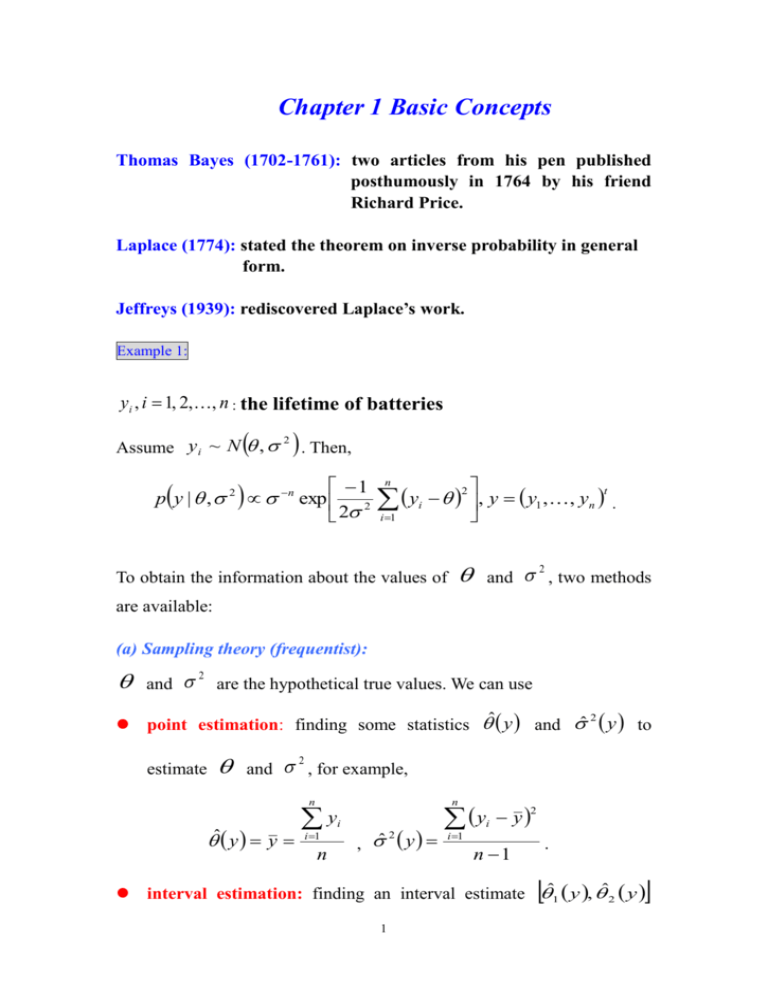
Chapter 1 Basic Concepts
Thomas Bayes (1702-1761): two articles from his pen published
posthumously in 1764 by his friend
Richard Price.
Laplace (1774): stated the theorem on inverse probability in general
form.
Jeffreys (1939): rediscovered Laplace’s work.
Example 1:
yi , i  1, 2,, n : the lifetime of batteries


2
Assume y i ~ N  ,  . Then,

p y |  ,
2
 
n
 1
exp  2
 2
n
 y
i 1
i
2
t
   , y   y1 , , yn  .

To obtain the information about the values of

and  , two methods
2
are available:
(a) Sampling theory (frequentist):

and 
2
are the hypothetical true values. We can use
2
 point estimation: finding some statistics ˆ y  and ˆ  y  to
estimate

and  , for example,
2
n
ˆ y   y 
y
i 1
n
n
i
2
, ˆ  y  
 y
i 1
 y
2
i
n 1
.


 interval estimation: finding an interval estimate ˆ1  y , ˆ2  y 
1
and ˆ12  y , ˆ 22  y  for
estimate for

and  , for example, the interval
2
,

s
s  
   , Z ~ N (0,1).
y

z
,
y

z
,
P
Z

z






2
2
2
2
n
n 

(b) Bayesian approach:

2
Introduce a prior density   , 
 for

and  . Then, after some
2
manipulations, the posterior density (conditional density given y)


f  ,  2 | y can be obtained. Based on the posterior density, inferences
about

and 
2
can be obtained.
Example 2:
X ~ b10, p  : the number of wins for some gambler in 10 bets,
where p is the probability of winning.
Then,
10 
10 x
f x | p     p x 1  p  , x  1,2, ,10.
x
(a) Sampling theory (frequentist):
To estimate the parameter p, we can employ the maximum likelihood
principle. That is, we try to find the estimate
p̂
to maximize the
likelihood function
10  x
10 x
l  p | x   f x | p     p 1  p  .
x
2
x  10 ,
For example, as
Thus,
10 
1010
l  p | x   l  p | 10    p10 1  p 
 p10 .
10 
ˆ  1 . It is a sensible estimate. Since we can win all the
p
time, the sensible estimate of the probability of winning should be 1. On
the other hand, as
Thus,
x  0,
10 
100
10
l  p | x   l  p | 0    p 0 1  p   1  p  .
0
ˆ  0 . Since we lost all the time, the sensible estimate of
p
the probability of winning should be 0. In general, as
ˆ 
p
xn,
n
, n  0,1,,10,
10
maximize the likelihood function.
(b) Bayesian approach::
  p  : prior density for p, i.e., prior beliefs in terms of probabilities of
various possible values of p being true.
Let
  p 
r a  b  a 1
b 1
p 1  p 
 Beta a, b  .
r a r b 
Thus, if we know the gambler is a professional gambler, then we can use
the following beta density function,
  p  2 p  Beta2,1 ,
to describe the winning probability p of the gambler.
The plot of the density function is
3
1.0
0.0
0.5
prior
1.5
2.0
Beta(2,1)
0.0
0.2
0.4
0.6
0.8
1.0
p
Since a professional gambler is likely to win, higher probability is
assigned to the large value of p.
If we know the gambler is a gambler with bad luck, then we can use the
following beta density function,
  p  21  p  Beta1,2 ,
to describe the winning probability p of the gambler. The plot of the
density function is
1.0
0.0
0.5
prior
1.5
2.0
Beta(1,2)
0.0
0.2
0.4
0.6
0.8
1.0
p
Since a gambler with bad luck is likely to lose, higher probability is
4
assigned to the small value of p.
If we feel the winning probability is more likely to be around 0.5, then we
can use the following beta density function,
  p  6 p1  p  Beta2,2 ,
to describe the winning probability p of the gambler. The plot of the
density function is
0.0
0.5
prior
1.0
1.5
Beat(2,2)
0.0
0.2
0.4
0.6
0.8
1.0
p
If we don’t have any information about the gambler, then we can use the
following beta density function,
  p   1  Beta1,1 ,
to describe the winning probability p of the gambler. The plot of the
density function is
1.0
0.9
0.8
prior
1.1
1.2
Beta(1,1)
0.0
0.2
0.4
0.6
p
5
0.8
1.0
posterior density of p given x  conditiona l density of p given x
f x, p  joint density of x and p
 f  p | x 

f x 
marginal density of x
f  x | p   p 

 f x | p   p   l  p | x   p 
f x 
Thus, the posterior density of p given x is
f  p | x     p l  p | x  
r a  b  a 1
b 1  n 
n x
p 1  p    p x 1  p 
r a r b 
 x
 ca, b, x  p x a 1 1  p 
b 10 x 1
In fact,
r a  b  10 
b 10 x 1
p xa 1 1  p 
r  x  a r b  10  x 
 Beta x  a, b  10  x 
f  p | x 
Then, we can use some statistic based on the posterior density, for
example, the posterior mean
E  p | x    pf  p | x dp 
1
0
As
xa
a  b  10 .
xn,
ˆ  E  p | n 
p
an
a  b  10
is different from the maximum likelihood estimate
n
10 .
Note:
f  p | x     p l  p | x 
 the original informatio n about p the informatio n from the data 
 the new informatio n about p given the data
6
Properties of Bayesian Analysis:
1. Precise assumption will lead to consequent inference.
2. Bayesian analysis automatically makes use of all the information from
the data.
3. The inferences unacceptable must come from inappropriate assumption
and not from inadequacies of the inferential system.
4. Awkward problems encountered in sampling theory do not arise.
5. Bayesian inference provides a satisfactory way of explicitly
introducing and keeping track of assumptions about prior knowledge or
ignorance.
7