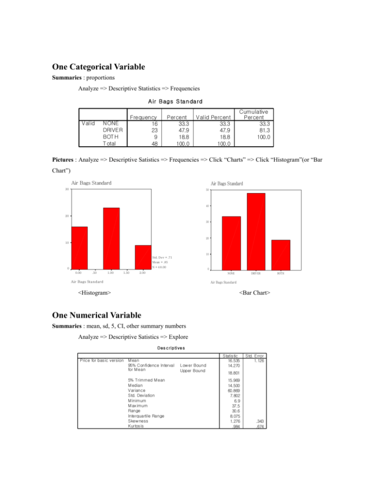
One Categorical Variable
Summaries : proportions
Analyze => Descriptive Statistics => Frequencies
A ir Bags S ta n da rd
Valid
Frequency
16
23
9
48
NONE
DRIVER
BOT H
T otal
Percent
33.3
47.9
18.8
100.0
Valid Percent
33.3
47.9
18.8
100.0
Cumulative
Percent
33.3
81.3
100.0
Pictures : Analyze => Descriptive Satistics => Frequencies => Click “Charts” => Click “Histogram”(or “Bar
Chart”)
Air Bags Standard
Air Bags Standard
30
50
40
20
30
20
10
Std. Dev = .71
Percent
Frequency
10
Mean = .85
N = 4 8.00
0
0.00
.50
1.00
1.50
2.00
0
NONE
Air Bags Sta ndard
DRIV ER
Air Bags Standard
<Histogram>
<Bar Chart>
One Numerical Variable
Summaries : mean, sd, 5, CI, other summary numbers
Analyze => Descriptive Satistics => Explore
Des c ripti ve s
Price for basic version
M ean
95% Confidence Interval
for M ean
5% Trimmed M ean
M edian
Variance
Std. Deviation
M inimum
M ax imum
Range
Interquartile Range
Skewness
Kurtosis
Lower Bound
Upper Bound
Statistic
16.535
14.270
Std. Error
1.126
18.801
15.969
14.500
60.869
7.802
6.9
37.5
30.6
8.075
1.276
.984
.343
.674
BOTH
P er ce n til es
5
Weighted
Average(Definition 1)
T ukey 's Hinges
Price for basic version
10
7.900
8.380
Price for basic version
Percentiles
50
25
75
90
95
11.400
14.500
19.475
33.030
34.510
11.400
14.500
19.450
Analyze => Descriptive Statistics => Explore => Click “Plots” =.> Click “stem-and
Pictures :
leaf”,”histogram”
Or Graphs => Interactive => Histogram or Box plot
40
40%
48
47
46
45
44
30
30%
Percent
20
20%
10
10%
0
N=
10.0
20.0
30.0
48
Price for basic vers
Price for basic version
<Histogram>
<Box-Plot>
Price for basic version Stem-and-Leaf Plot
Frequency
Stem &
Leaf
9.00
0 .
677888899
20.00
1 .
00111233333444444444
10.00
1 .
5578889999
2.00
2 .
02
2.00
2 .
69
5.00 Extremes
(>=33)
Stem width:
10.0
Each leaf:
1 case(s)
Notice that all 3 graphs indicates the data is skewed to the right which agrees with the
mean > median.
One Categorical and One Numerical Variable
Summaries :
mean and sd by group(categorical)
Analyze => Descriptive Statistics => Explore => Move “price” to dependent list => Move “airbag”
to factor list (it also gives histograms, stem-and-leaf plots and box plots)
Pictures : Graphs => Interactive => Histogram => Move “airbag” to Panel variable
Des c ripti ve s
Price for basic version
Air Bags Standard
NONE
DRIVER
M ean
95% Confidence Interval
for M ean
5% Trimmed M ean
M edian
Variance
Std. Deviation
M inimum
M ax imum
Range
Interquartile Range
Skewness
Kurtosis
M ean
95% Confidence Interval
for M ean
5% Trimmed M ean
M edian
Variance
Std. Deviation
M inimum
M ax imum
Range
Interquartile Range
Skewness
Kurtosis
M ean
95% Confidence Interval
for M ean
BOT H
Lower Bound
Upper Bound
Lower Bound
Upper Bound
Lower Bound
Upper Bound
5% Trimmed M ean
M edian
Variance
Std. Deviation
M inimum
M ax imum
Range
Interquartile Range
Skewness
Kurtosis
Statistic
9.781
8.766
10.796
9.763
9.300
3.630
1.905
6.9
13.0
6.1
3.150
.345
-1.169
15.909
14.910
.564
1.091
.482
16.908
15.834
14.800
5.338
2.310
13.3
19.9
6.6
4.200
.624
-1.270
30.144
25.571
.481
.935
1.983
34.718
30.294
33.000
35.398
5.950
20.1
37.5
17.4
10.050
-.673
-.841
<Histogram>
NO NE
Std. Error
.476
.717
1.400
<Box plot>
D RIV ER
100%
40
75%
Pe rce nt
50%
30
25%
20
0%
Price for basic version
BO T H
100%
75%
Pe rce nt
50%
25%
10
0
N=
16
23
9
NONE
DRIVE R
BOTH
0%
10.0
20.0
30.0
Pr ice for b a s ic v er s ion
Air Bags Stan dard
Two Categorical Variables
Summaries :
proportions by group
Data is 3 columns:
the (cell) counts by two categorial variables, row and col
where row are row categories, col are col categories and count is the number of observations in each row,col
Click on data, define weight cases by count variable then
Analyze => Descriptive statistics => Crosstabs => Click “Cells”
P as s en ger C a pa c ity * Ai r Ba gs Stan dar d C ros stabu la tion
NONE
Passenger
Capacity
NUM =2
NUM =4
NUM =5
NUM =6
NUm=7
NUM =8
T otal
Count
% within Passenger
Capacity
% within Air Bags
Standard
Count
% within Passenger
Capacity
% within Air Bags
Standard
Count
% within Passenger
Capacity
% within Air Bags
Standard
Count
% within Passenger
Capacity
% within Air Bags
Standard
Count
% within Passenger
Capacity
% within Air Bags
Standard
Count
% within Passenger
Capacity
% within Air Bags
Standard
Count
% within Passenger
Capacity
% within Air Bags
Standard
Air Bags Standard
BOT H
DRIVER
1
T otal
1
100.0%
100.0%
2.1%
4.3%
3
4
2
9
33.3%
44.4%
22.2%
100.0%
18.8%
17.4%
22.2%
18.8%
9
6
1
16
56.3%
37.5%
6.3%
100.0%
56.3%
26.1%
11.1%
33.3%
1
10
6
17
5.9%
58.8%
35.3%
100.0%
6.3%
43.5%
66.7%
35.4%
2
2
4
50.0%
50.0%
100.0%
12.5%
8.7%
8.3%
1
1
100.0%
100.0%
2.1%
6.3%
16
23
9
48
33.3%
47.9%
18.8%
100.0%
100.0%
100.0%
100.0%
100.0%
Pictures : Graphs => Interactive => Histogram => Click “airbag”(or “pass”) to Panel variable
NO NE
D RIV ER
75%
NUM= 2
NUM= 4
NUM= 5
NUM= 6
NUm = 7
NUM= 8
100%
75%
Pe rce nt
Pe rce nt
50%
25%
50%
25%
0%
0%
BO T H
75%
100%
75%
Pe rce nt
Pe rce nt
50%
25%
50%
25%
0%
3
4
5
6
Pa s s eng er C a pa city
7
0%
0.0
0.5
1.0
1.5
A ir B a g s Sta nd a r d
2.0
0.0
0.5
1.0
1.5
A ir B a g s Sta nd a r d
2.0
0.0
0.5
1.0
1.5
A ir B a g s Sta nd a r d
2.0
Two Numerical Variables
Summaries : means, etc by both variables, slope and intercept, correlation coefficient
Analyze => Descriptive Statistics => Explore => Move both variables to dependent list.
Des c ripti ve s
City M PG by EPA
rationgs
Price for basic version
M ean
95% Confidence Interval
for M ean
5% Trimmed M ean
M edian
Variance
Std. Deviation
M inimum
M ax imum
Range
Interquartile Range
Skewness
Kurtosis
M ean
95% Confidence Interval
for M ean
Statistic
20.85
19.69
Lower Bound
Upper Bound
Std. Error
.58
22.02
20.63
20.00
16.042
4.01
15
31
16
5.00
.912
.454
16.535
14.270
Lower Bound
Upper Bound
.343
.674
1.126
18.801
5% Trimmed M ean
M edian
Variance
Std. Deviation
M inimum
M ax imum
Range
Interquartile Range
Skewness
Kurtosis
15.969
14.500
60.869
7.802
6.9
37.5
30.6
8.075
1.276
.984
.343
.674
75
90
P er ce n til es
5
Weighted
Average(Definition 1)
T ukey 's Hinges
City M PG by EPA
rationgs
Price for basic version
City M PG by EPA
rationgs
Price for basic version
10
25
Percentiles
50
95
15.45
16.00
18.00
20.00
23.00
28.10
30.10
7.900
8.380
11.400
14.500
19.475
33.030
34.510
18.00
20.00
23.00
11.400
14.500
19.450
Analyze => Correlate => Bivariate => Move both variables to variables
C orre la ti on s
Price for
City M PG by
basic version EPA rationgs
Price for basic version Pearson Correlation
1.000
.872**
Sig. (2-tailed)
.
.000
N
48
48
City M PG by EPA
Pearson Correlation
.872**
1.000
rationgs
Sig. (2-tailed)
.000
.
N
48
48
**. Correlation is significant at the 0.01 level (2-tailed).
Analyze => Regression => Linear
C oe ffic ie ntsa
Standardi
z ed
Coefficie
nts
Beta
Unstandardized
Coefficients
B
Std. Error
-18.891
2.983
M odel
1
(Constant)
City M PG by
1.699
.141
EPA rationgs
a. Dependent Variable: Price for basic version
.872
t
-6.333
Sig.
.000
12.088
.000
95% Confidence Interval for B
Lower Bound Upper Bound
-24.896
-12.887
1.416
1.982
Pictures : Graphs => Interactive => Scatter plot => Plot X vs Y with regression line

Linear Regression




Pri ce for basic versio n
30.0



20.0






10.0


15














Pr ice for b a s ic v er s ion = -18.89 + 1.70 * citympg
R -Squa r e = 0.76







20
25
City MPG by EPA rationgs
30