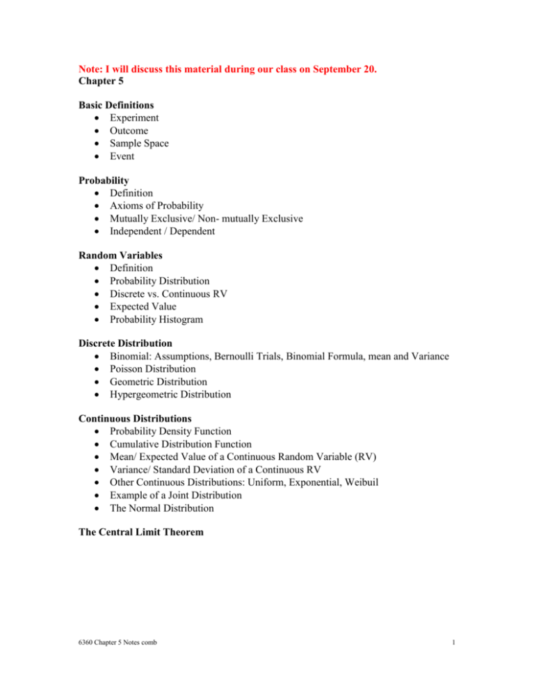
Note: I will discuss this material during our class on September 20.
Chapter 5
Basic Definitions
 Experiment
 Outcome
 Sample Space
 Event
Probability
 Definition
 Axioms of Probability
 Mutually Exclusive/ Non- mutually Exclusive
 Independent / Dependent
Random Variables
 Definition
 Probability Distribution
 Discrete vs. Continuous RV
 Expected Value
 Probability Histogram
Discrete Distribution
 Binomial: Assumptions, Bernoulli Trials, Binomial Formula, mean and Variance
 Poisson Distribution
 Geometric Distribution
 Hypergeometric Distribution
Continuous Distributions
 Probability Density Function
 Cumulative Distribution Function
 Mean/ Expected Value of a Continuous Random Variable (RV)
 Variance/ Standard Deviation of a Continuous RV
 Other Continuous Distributions: Uniform, Exponential, Weibuil
 Example of a Joint Distribution
 The Normal Distribution
The Central Limit Theorem
6360 Chapter 5 Notes comb
1
INTRODUCTION TO PROBABILITY
Information in the Appendix. See if you can do any of these problems – we will discuss
in our next class.
1. An experiment consists of drawing one car from a deck of 52 cards. What is the
probability of
a) a red card
b) an ace
c) a king
d) a king or an ace
e) a red card or a king
2. An experiment consists or drawing two cards with replacement. What is the
probability of:
a) a king on the first draw and a jack on the second
b) a three on the first and a nine on the second?
3. An experiment consists or drawing two cards without replacement. What is the
probability of:
a) a king on the first draw and a jack on the second
b) a king on both draws?
4. A bin contains 5 aluminum, 2 steel and 3 brass parts. Three parts are selected. Find
the probability that they are drawn in the order brass, aluminum, steel. What is the
probability that 2 are aluminum and 1 is brass?
5. The probability that an integrated circuit chip will have a defective etching is 0.12;
the probability that it will have a crack defect is 0.29, and the probability that it has
both defects is 0.07.
a) What is the probability that a newly manufactured chip will have either an
etching or a crack defect?
b) What is the probability that a new chip will have neither defect?
6360 Chapter 5 Notes comb
2
PROBABILITY DISTRIBUTIONS
Random Variable - Maps a real number to the outcome of an experiment
Two Types of Random Variables
1. Discrete
the random variable assumes discrete (countable) values
2. Continuous
the random variable can assume values represented by a
continuous interval of numbers
Examples of Discrete Random Variable
 the number of automobile accidents in Houston.
 the number of building permits issued by the city during the last year
 the number of power failures per month
 the number of defective parts produced in a manufacturing operation
Examples of Continuous Random Variable
 force required to break a certain tensile specimen
 voltage
 distance
Probability Distribution for a Random Variable
Assigns probabilities to the possible outcomes as measures of the likelihood that the
various numerical values will occur
Probability Function for a Discrete Random Variable
 For a discrete random variable X with possible outcomes of x1, x2, …., the probability
function is a nonnegative function f(x) such that f(x) = P[X = x].
 Note that the probability function of a discrete random variable is often expressed
using a table.
 Properties:
 f(x) assumes values between 0 and 1 (inclusive)
 the f(x) values sum to 1
Cumulative Probability Function
Assume X is a random variable. The function F(x) = P[X < x].
Note for a discrete random variable, F(x) = f(z) over z < x
Mean or Expected Value of a Discrete RV
E(X) = x * f(x)
E(X) = X1*P(X1) + …. + Xn*P(Xn)
Variance/Standard Deviation of a Discrete RV
Var (X) = (x - EX)2 *f(x) = x2 *f(x) - EX2
6360 Chapter 5 Notes comb
3
Example of a Discrete Random Variable
Let X = the number of imperfections in a roll of sheet metal.
Suppose X has the following probability distribution.
Probability Distribution of the Number of Imperfections
x
0
1
2
3
4
f(x)
0.40
0.30
0.15
0.10
0.05
1.00
Note that the sum of the probabilities is 1. f(x) = 1
The random variable X assumes the number of imperfection found, i.e. there can be
0,1,2,3, or 4 imperfections on the roll.
We formed a probability distribution by assigning probabilities to each of these
outcomes. For example
f(2) = P[X = 2] = 0.15
Cumulative Probability Distribution of Number of Imperfections
x
0
1
2
3
4
f(x) = P[X = x]
0.40
0.30
0.15
0.10
0.05
F(x) = P(X  x)
0.40
0.70
0.85
0.95
1.00
Note: F(3) = P[X < 3] = P[X < 2] = f(0) + f(1) + f(2) = 0.4 + 0.3 + 0.15 = 0.85
The expected value of a random variable is:
E(X) = x f(x) = 0*.4 + 1*.3 + 2*.15 + 3*.1 + 4*.05
= 0 + 0.3 + 0.3 + 0.3 + 0.2 = 1.1
On the average we expect the number of imperfections to be 1.1.
The variance of the random variable is:
Var (X) = (x - EX)2 * f(x)
Var (X) = x2 * f(x) - EX2
6360 Chapter 5 Notes comb
4
Example: Probability Histogram
X = # of equipment failures in a one month period
In the following example, the number of equipment failures can take on a value from 0 to 9.
The probability distribution on the left lists each possibility with the associated probability that
it will occur. The cumulative function is also shown.
Equipment Failures
E Q U IP M E N T F A IL U R E S
IN O N E -M O N T H
0.3
6360 Chapter 5 Notes comb
0.2
0.15
0.1
0.05
9
8
7
6
5
0
4
2
6
6
6
9
4
3
2
1
1
1
3
.1
.2
.2
.1
.0
.0
.0
.0
.0
.0
0.25
2
0
0
0
0
0
0
0
0
0
0
F (X )
0 .1 2
0 .3 8
0 .6 4
0 .8
0 .8 9
0 .9 3
0 .9 6
0 .9 8
0 .9 9
1
1
f(x )
0
X
0
1
2
3
4
5
6
7
8
9
5
SOME DISCRETE PROBABILITY DISTRIBUTIONS
Binomial Distribution
The Binomial Distribution assumes the following
 An experiment is performed a finite number of times.
 Each outcome of the experiment can result in ‘success’ or ‘failure.’
 There is a constant probability of success (and we will label it p) and a
probability of failure (q = 1 - p).
 The trials of the experiment are independent,
 X is the number of successes in n trial of the experiment
Examples





number of defective parts
number of projects that meet specifications
number of employees that passed the training
number of nonconforming transducers
number of containers that are over filled
Probability Function for the Binomial
The binomial distribution has the following probability function
X = the number of successes in n independent Bernoulli trials of an experiment
f(x) = nCxpx * (1-p)n - x
for x = 0,1,2….n
f(x) = 0
otherwise
Example of the Binomial
A manufacturer claims that only 10% of his machines require repair within one year.
Find the probability of 5 repairs from 20 machines.
Use the Binomial formula to determine the probability of 5 repairs (i.e. successes) in 20
trials of the experiment.
n = 20
x= 5
20C5
= 20!/5!* (20 – 5)! = 15,504
px = (0.1)5 = 0.00001
p = 0.10
q = 1 – 0.10 = 0.90
(1- p)n - x = (0.9)15 = 0.20589
P(X = 5) = 15504*0.00001*0.20589= 0.0319
6360 Chapter 5 Notes comb
6
Poisson Distribution
The Poisson distribution counts the number of relatively rare events over a specified
interval of space or time,
Examples of the Poisson
 the number of flaws in a length of wire
 the number of particles of contamination that occur on a storage disk
 the number of messages arriving for routing through a switching center in a
communications network
 the number of imperfections in a bolt of cloth
 the number of arrivals at a retail outlet
Probability Function for the Poisson
X = # of success in an interval of time, space, distance
f(x) = e-x/x!
for x = 0,1,2,…...
f(x) = 0
otherwise
Example of Poisson
Tin plates that are produced by a continuous electrolytic process are inspected. The
number of imperfections spotted per minute is 0.2. Find the probability of 1 imperfection
in 3 minutes.
e = 2.718…
x=1
 = 0.2 * 3 = 0.6
(If there are 0.2 imperfections in 1 minute, we have 0.6 imperfections in 3 minutes.)
f(1) = (e-1)/1! = 0.329287
Geometric Distribution
This distribution is similar to the Binomial, but it counts the number of trials to the first
success.
Probability Function for the Geometric
X = # of trials until the first success
f(x) = px(1-p)n-x
for x = 0,1,2….n
f(x) = 0
otherwise
Example of the Geometric Distribution
The probability that a measuring device will show excessive drift is 0.05. A series of
devices is tested. What is the probability that the 6th device will show excessive drift?
Find the probability of the 1st drift on the 6th trail.
P(X = 6) = (0.05)*(0.95)5 = 0.039
6360 Chapter 5 Notes comb
7
Discrete Probability Distributions
1. Human error is the reason for 75% of all accidents in a plant. Find the probability that
human error will be reported as the reason for two of the next four accidents. [27/128]
2. During one stage in the manufacture of integrated circuit chips, a coating must be
applied. If 70% of the chips receive a thick enough coating, find the probabilities that
among 15 chips:
2.1
at least 12 will have a thick enough coating [0.2969]
2.2
at most 6 will have a thick enough coating [0.0152]
2.3
exactly 10 will have a thick enough coating [0.2061]
3. The probability that the noise level of a wide band amplifier will exceed 2 dB is 0.05.
for a group of 12 amplifiers, find:
3.1
one will exceed 2 dB
3.2
at most two will exceed 2 dB
3.3
two or more will exceed 2 dB
1. Given that the switch board of a consultants office receives on the average 0.6 calls
per minute, find the probability that:
4.1
in a given minute, there will be at least one call
4.2
in a 4-minute interval, there will be at least three calls
2. At a check out counter, customers arrive at an average rate of 1.5 per minute. Find the
probability that:
5.1
at most four will arrive in any given minute [0.981]
5.2
at least three will arrive during an interval of 2 minutes [0.577]
5.3
at most 15 will arrive during an interval of 6 minutes. [0.978]
6360 Chapter 5 Notes comb
8
Binomial and Poisson / Minitab
Binomial
Use Calc/Probability Distributions/Binomial
MTB >
MTB >
MTB >
SUBC>
# Binomial
#P = 0.05 and N = 16
CDF;
Binomial 16 .05.
Cumulative Distribution Function
Binomial with n = 16 and p = 0.0500000
x
0
1
2
3
4
5
6
P( X <= x )
0.4401
0.8108
0.9571
0.9930
0.9991
0.9999
1.0000
MTB > # Inverse Binomial
MTB >
MTB > INVCDF .1247;
SUBC> Binomial 16 .05.
Inverse Cumulative Distribution Function
Binomial with n = 16 and p = 0.0500000
x
0
P( X <= x )
0.0000
x
0
P( X <= x )
0.4401
Poisson
MTB > # Poisson with mean of 5
MTB >
MTB > CDF;
SUBC> Poisson 5.
Cumulative Distribution Function
Poisson with mu = 5.00000
x
0
1
2
3
4
5
6
7
8
9
10
11
12
13
14
15
16
P( X <= x )
0.0067
0.0404
0.1247
0.2650
0.4405
0.6160
0.7622
0.8666
0.9319
0.9682
0.9863
0.9945
0.9980
0.9993
0.9998
0.9999
1.0000
6360 Chapter 5 Notes comb
9
CONTINUOUS RANDOM VARIABLES
A continuous random variable can assume values represented by a continuous interval of
numbers
Examples
 current in a copper wire (variation from current source, temperature
change…)
 diameter of a bolt (variation from calibration, tool wear, raw materials…)
 time to complete a machining operation
 length of time to play a set of badminton
 heights, weights, lengths, etc,
Note the probability of selecting exact values cannot be measured; instead we are
concerned with the probability of an interval of values, and tabular forms are no
longer possible. Instead we use a function, referred to as the probability density
function.
Probability Density Function
The function f(x) is a probability density function for the continuous random
variable X, defined over the real numbers R if:
f(x) > 0
for all x that are elements of R

 f(x)dx
=1

b
P(a < x < b) >
 f(x)dx
a
Note that consequence of X being a continuous random variable is that
P(X =x) = 0
and when evaluating the probability of an interval, it is not necessary to consider
the equality sign i.e. P(a < X < b) = P(a < X < b).
Example
The lead concentration in gasoline ranges from 0.2 to 0.6 grams per liter. Define the
random variable X.
X:
grams of lead per liters
The density of the random variable is given by
f(x) = kx - 1 for 0.2 < x < 0.6
f(x) = 0
otherwise
a)
Find the value of k.
6360 Chapter 5 Notes comb
10
b)
What is the probability that a liter of gas will have between .3 and .5 grams of
lead?
[Ref. Milton and Arnold]
Solution
According to the definition

(kx-1)dx
=1



 0dx
+


(kx-1)dx

+  0dx
=1

Cumulative Distribution Function
An alternate way of describe a continuous random variable is the cumulative distribution
function (cdf).
Assume X is a random variable. The function
F(x) =
P[X < x]
x
 f(x) dx
for  x

Example B
For the distribution function of Example a, find the cumulative density function.
Mean or Expected Value of a Continuous RV

E(X) =

x f(x)dx
Variance/Standard Deviation of a Continuous RV

Var (X) = (x - E(X))2 f(x)dx

6360 Chapter 5 Notes comb
11
NORMAL DISTRIBUTIONS
•
•
•
Family of distributions, all with the same general shape.
Symmetric about the mean
The y-coordinate (height) specified in terms of the mean and the standard deviation of
the distribution
Normal Probability Density
For all x
f ( x) 
1
( x   )2 / 2  2
e
2
Standard Normal Distribution
The normal distribution with  =0 and  =1 is called the standard normal.
For all x:
f (t ) 
1
2
e t / 2
2
Transformations
Normal distributions can be transformed to the standard normal.
We use what is called the z-score, which is a value that gives the number of standard
deviations that X is from the mean.
Standard Normal Table
Use the table in the text to verify the following.
1. P(z < -2) = F(2) = 0.0228
2. F(2) = 0.9773
3. F(1.42) = 0.9222
4. F(-0.95) = 0.1711
6360 Chapter 5 Notes comb
12
Example of the Normal
The amount of instant coffee that is put into a 6 oz jar has a normal distribution with a
standard deviation of 0.03. oz. What proportion of the jar contain:
a) Less than 6.06 oz?
b) More than 6.09 oz?
c) Less than 6 oz?
Normal Example - part a)
Assume = 6 and  = 0.03.
The problem requires us to find
P(X < 6.06)
Convert x = 6.06 to a z-score
z = (6.06 - 6)/.03 = 2
and find:
P(z < 2) = .9773
So 97.73% of the jars have less than 6.06 oz.
Normal Example - part b)
Again = 6 and  = 0.03.
The problem requires us to find:
P(X > 6.09)
Convert x = 6.09 to a z-score
z = (6.09 - 6)/.03 = 3
and find
P(z > 3) = 1- P(x < 3) = 1- .9987= 0.0013
So 0.13% of the jars have more than 6.09oz.
6360 Chapter 5 Notes comb
13
Normal Distribution/ MTB
MTB > # Use Calc\Probability Distributions
MTB > # Normal Distribution
MTB > CDF -1.77;
SUBC>
Normal 0.0 1.0.
Cumulative Distribution Function
Normal with mean = 0 and standard deviation = 1.00000
x
-1.7700
P( X <= x )
0.0384
MTB > PDF -1.77;
SUBC>
Normal 0.0 1.0.
Probability Density Function
Normal with mean = 0 and standard deviation = 1.00000
x
-1.7700
f( x )
0.0833
MTB > InvCDF .0833;
SUBC>
Normal 0.0 1.0.
Inverse Cumulative Distribution Function
Normal with mean = 0 and standard deviation = 1.00000
P( X <= x )
0.0833
x
-1.3832
MTB >
6360 Chapter 5 Notes comb
14
CENTRAL LIMIT THEOREM
 specifies a theoretical distribution
 formulated by the selection of all possible random samples of a fixed size n
 a sample mean is calculated for each sample
Sampling Distribution Of The Mean
 The mean of the sample means is equal to the mean of the population from which the
samples were drawn.
 The variance of the distribution is  divided by the square root of n. (the standard
error.)
Standard Error
Standard Deviation for the Distribution of Sample Means
x 

n
Central Limit Theorem
1. Consider a population with mean  and standard deviation .
2. Draw a random sample of n observations from this population where n is a large
number (n> 30).
3. Find the mean x for each and every sample.
4. The distribution of the sample means x will be approximately normal. This
distribution is called the Sampling Distribution of the Means or the Distribution of
Sample Means.
5. The mean and standard deviation (called the standard error) of the Distribution of
Sample Means is:
6.
x  
The mean of the Sampling Distribution equals the mean of the Population
x 
The standard error equals the standard deviation of the population divided by the
square root of the sample size.

n
The approximation becomes more accurate as n becomes large.
6360 Chapter 5 Notes comb
15
Example of CLT
A certain brand of tires has a mean life of 25,000 miles with a standard deviation of 1600
miles. What is the probability that the mean life of 64 tires is less than 24,600 miles?
Solution
The sampling distribution of the means has a mean of 25,000 miles (the population mean)
 = 25,000 mi.
and a standard deviation (i.e. standard error) of
 x = 1600/8 = 200
Convert 24,600 mi. to a z-score and use the normal table to determine the required
probability.
z = (24,600 – 25,000)/200 = -2
P(z < -2) = 0.0228
or 2.28% of the sample means will be less than 24,600 mi.
6360 Chapter 5 Notes comb
16
Distribution of Individual Values for 6 Samples from a Population with an
Exponential Distribution
30
Frequency
Frequency
30
20
10
0
20
10
0
0.0
0.5
1.0
1.5
2.0
2.5
3.0
3.5
4.0
4.5
5.0
0.0
0.5
1.0
1.5
2.0
C25
2.5
3.0
3.5
4.0
4.5
5.0
C12
35
30
30
Frequency
Frequency
25
20
15
10
20
10
5
0
0
0
1
2
3
4
5
6
0
1
2
C1
3
4
5
6
C10
35
40
30
30
Frequency
Frequency
25
20
15
10
20
10
5
0
0
0
1
2
3
4
5
6
0
C1
1
2
3
4
5
6
C30
Distribution of the Means of 30 Samples
35
30
Frequency
25
20
15
10
5
0
0.5
1.0
1.5
C31
6360 Chapter 5 Notes comb
17