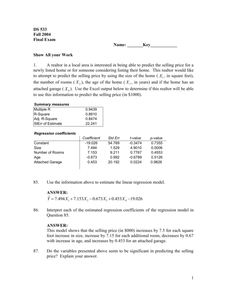
DS 533
Fall 2004
Final Exam
Name: _______Key____________
Show All your Work
1.
A realtor in a local area is interested in being able to predict the selling price for a
newly listed home or for someone considering listing their home. This realtor would like
to attempt to predict the selling price by using the size of the home ( X1 , in square feet),
the number of rooms ( X 2 ), the age of the home ( X 3 , in years) and if the home has an
attached garage ( X 4 ). Use the Excel output below to determine if this realtor will be able
to use this information to predict the selling price (in $1000).
Summary measures
Multiple R
R-Square
Adj. R-Square
StErr of Estimate
0.9439
0.8910
0.8474
22.241
Regression coefficients
Constant
Size
Number of Rooms
Age
Attached Garage
85.
Coefficient
-19.026
7.494
7.153
-0.673
0.453
Std Err
54.769
1.529
9.211
0.992
20.192
t-value
-0.3474
4.9010
0.7767
-0.6789
0.0224
p-value
0.7355
0.0006
0.4553
0.5126
0.9826
Use the information above to estimate the linear regression model.
ANSWER:
Yˆ  7.494 X1  7.153 X 2  0.673 X 3  0.453 X 4 19.026
86.
Interpret each of the estimated regression coefficients of the regression model in
Question 85.
ANSWER:
This model shows that the selling price (in $000) increases by 7.5 for each square
foot increase in size, increase by 7.15 for each additional room, decreases by 0.67
with increase in age, and increases by 0.453 for an attached garage.
87.
Do the variables presented above seem to be significant in predicting the selling
price? Explain your answer.
1
ANSWER:
No; the only variable that is significant in this model is the size of the home in
square feet (p-value=0.0006). The other variables are not significant.
88.
Would any of the variables in this model be considered a dummy variable?
Explain your answer.
ANSWER:
Yes; the attached garage is a dummy (0, 1) variable. This is a yes or no response.
89.
Identify and interpret the coefficient of determination ( R2 ) and the standard error
of the estimate (se) for the model in Question 85.
ANSWER:
R2 = 0.8910; This represents 89.1% of the variation in the selling price can be
explained by this regression equation. se = 22.241; This represents the standard
deviation of the residuals.
90.
Would you recommend that the realtor use this model to predict the selling price
of a home? Would you want to make any changes to this model before using it to
predict the selling price of a home? Explain.
ANSWER:
The size of the home has a fairly strong relationship with the selling price, but the
other variables do not seem to be significant in predicting the selling price. If you
want to consider another variable, the appraised value of the home may be useful.
However, you may also want to consider if there is multicollinearity exists in this
model. In the current model it would seem as though the size of the home and the
number of rooms could be highly correlated with one another. This could cause
some problems with predicting the selling price of the home.
Give a 95% confidence interval for the average selling price for
2
2.
Below you will find a regression model that compares the relationship between
the average utility bill (Y, in $) for homes of a particular size and the average monthly
temperature (X, in Fahrenheit). The data represents monthly values for the past year.
Also, the value for the Durbin-Watson statistic = 1.244, and a residual plot is shown
below.
Summary measures
Multiple R
R-Square
StErr of Estimate
0.0295
0.0009
24.8184
ANOVA table
Source
Explained
Unexplained
df
1
10
SS
MS
5.3575
5.3575
6159.5125 615.9512
F
0.0087
p-value
0.9275
Regression coefficients
Coefficient
112.547
0.0403
Constant
Average Monthly Temp
Std Err
28.815
0.4316
t-value
3.9059
0.0933
p-value
0.0029
0.9275
40
30
20
10
0
-10
1
2
3
4
5
6
7
8
9
10
11
12
-20
-30
-40
48.
Estimate the regression model. How well does this model fit the given data?
ANSWER:
Yˆ = 0.0403 X1 + 112.547; this is not a very good fit. The R2 = 0.0009.
49.
Is there a linear relationship between X and Y? Explain how you arrived at your
answer.
ANSWER:
3
No; The p-value = 0.9275 for the F-statistic. There is not a significant linear
relationship between these two variables.
50.
In looking at the graph of the residuals, do you see any evidence of any violations
of the assumptions regarding the errors of the regression model?
ANSWER:
There seems to be a pattern to the residuals and this violates the assumption that
the residuals are probabilistically independent. The data appears to be
autocorrelated.
51.
Giving the Durbin-Watson value presented above, what would you conclude
about the data?
ANSWER:
The Durbin-Watson statistic = 1.244 seems to indicate that there is lag 1
autocorrelation present in this data. This value indicates positive autocorrelation
in the data.
52.
Given you answer in Question 51, would you recommend modifying the original
regression model? If so, how would you modify it?
ANSWER:
There is not an easy fix to the autocorrelation problem. In this case, you could
use the average temperature to predict the next month’s utility bill. Also, you
could look for other variables that may affect the utility bill such as appliances in
house, number of people living in house, whether house has central air/heat, etc.
You may be able to identify another variable that has a linear relationship with the
average utility bill.
4
3.
TOD Chevy is using Holt’s Method to forecast weekly car sales. Currently, the level is
estimated to be 50 cars per week, and the trend is estimated to be 6 cars per week. During
the current week 30 cars are sold. Forecast the number of cars 3 weeks from now.  = 
=0.3.
3.
The following specific percentage seasonal Factors are given for the month of December:
75.4,
86.8,
96.9,
72.6,
80.0,
85.4
Assume multiplicative decomposition model. If the expected trend-cycle for December is
$900, and the mean seasonal Factors is used, what is the forecast for December?
5
Multiple Choice Questions
Select the best answer
1.
2.
If you are going to use a regression equation for prediction, you hope to have a
reasonably
se .
R2 and a reasonably
a. small; large
b. large; small
c. small; small
d. large; large
e. none of the above
ANSWER: b
In choosing the “best-fitting” line through a set of points in linear regression, we
choose the one with the:
a.
b.
c.
d.
e.
3.
In a multiple regression analysis, there are 20 data points and 3 independent
variables, and the sum of the squared differences between observed and predicted
values of y is 160. The multiple standard error of estimate will be:
a.
b.
c.
d.
e.
4.
smallest sum of squared residuals
largest sum of squared residuals
smallest number of outliers
largest number of points on the line
none of the above
3.162
10
9.41
8.42
none of the above
The F-ratio from the ANOVA table is calculated by:
a. MSR / MSE
b. MSE / MSR
c. SST / SSE
d. SSR / SSE
e. none of the above
ANSWER: a
5.
The
a.
b.
c.
d.
can be used to test for autocorrelation.
regression coefficient
correlation coefficient
Durbin-Watson statistic
F-test
6
e. t-test
ANSWER:
5.
A multiple regression equation includes 6 independent variables, and the
coefficient of multiple determination is 0.91. The percentage of the variation in y
that is explained by the regression equation is:
a.
b.
c.
d.
e.
6.
c
91%
95%
83%
about 15%
none of the above
In regression analysis, multicollinearity refers to:
a. the response variables being highly correlated
b. the explanatory variables being highly correlated
c. the response variable(s) and the explanatory variable(s) are highly correlated
with one another
d. the response variables are highly correlated over time.
e. none of the above
ANSWER: b
7.
When determining whether to include or exclude a variable in regression analysis,
if the p-value associated with the variable’s t-value is above some accepted
significance value, such as 0.05, then:
a. the variable is a candidate for inclusion
b. the variable is a candidate for exclusion
c. the variable is redundant
d. the variable does not fit the guidelines of parsimony
e. none of the above
ANSWER: b
8.
The following are the values of a time series for the first four time periods:
t
yt
1
24
2
25
3
26
4
27
Using a three-period moving average, the forecasted value for time period
5 is:
a.
b.
c.
d.
20.4
25.5
26
none of the above
7
9.
When using exponential smoothing, a smoothing constant must be used. The
smoothing constant is a value that:
a.
b.
c.
d.
ranges between 0 and 1
ranges between –1 and +1
is equal to the largest observed value in the series
represents the strength of the association between the forecasted and observed
values
e. none of the above
10.
Winter’s model differs from simple exponential smoothing in that it includes a
term for:
a. seasonality
b. trend
c. residuals
d. cyclical fluctuations
e. none of the above
Questions 11, through 14 refer to the following table.
Seasonal Indexes of sales revenue of People's Bank are:
January
February
March
April
May
June
July
August
September
October
November
December
11.
Total revenue for People's Bank in 1999 is forecasted to be $60,000. Based on the
seasonal indexes above, sales in the first three months of 1999 should be:
a.
b.
c.
d.
e.
12.
1.20
.90
1.00
1.08
1.02
1.10
1.05
.90
.85
1.00
1.10
.80
$4,800
$15,500
$14,723
$13,500
None of the above.
If December 1999 revenue for People's Bank amounted to $5,000, a reasonable estimate
of revenue for January 2000, based on the seasonal indexes given above would be:
8
a.
b.
c.
d.
f.
13.
14.
$3,000
$4,500
$4,800
$7,500
None of the above.
If revenue of People's Bank amounted to $5,500 in November 1999; the November 1999
sales revenue, after adjustment for seasonal variation using the indexes given above,
would be:
a.
$6,500
b.
$6,050
c.
$5,500
d.
$4,500
e.
None of the above.
Suppose that a simple exponential smoothing model is used (with  = 0.40) to
forecast monthly sandwich sales at a local sandwich shop. The forecasted
demand for September was 1560 and the actual demand was 1480 sandwiches.
Given this information, what would be the forecast for October in number of
sandwiches?
a.
b.
c.
d.
e.
1480
1528
1560
1592
cannot be determined from the information given
15.
Which of the following is not an attribute of a normal probability distribution?
16.
a.
It is symmetrical about the mean.
b.
Most observations cluster around the mean.
c.
Most observations cluster around zero.
d.
The distribution is completely determined by the mean and variance.
e.
All the above are correct.
When a time series contains no trend, it is said to be
a.
b.
c.
d.
e.
17.
nonstationary.
seasonal.
nonseasonal.
stationary.
filtered.
The difference between seasonal and cyclical components is:
a.
b.
Duration.
Source.
9
18.
19.
20.
21.
22.
c.
Predictability.
d.
Frequency.
e.
All the above.
A linear trend means that the time series variable changes by:
a. a constant amount each time period
b. a constant percentage each time period
c. a positive amount each time period
d. a negative amount each time period
e. none of the above
ANSWER: a
When using the moving average method, you must select
represent(s) the number of terms in the moving average.
which
a. a smoothing constant
b. the explanatory variables
c. an alpha value
d. a span
e. none of the above
ANSWER: d
The forecast error is:
a. the difference between this period’s value and the next period’s value
b. the difference between the average value and the expected value of the
response variable
c. the difference between the explanatory variable value and the response
variable value
d. the difference between the actual value and the forecast
e. none of the above
ANSWER: d
A regression approach can also be used to deal with seasonality by using
variables for the seasons.
a. smoothing
b. response
c. residual
d. dummy
e. none of the above
ANSWER: d
In a random series, successive observations are independent of one another. If
this property is violated, the observations are said to be:
a.
b.
c.
d.
autocorrelated
intercorrelated
causal
seasonal
10
e. none of the above
ANSWER: a
11