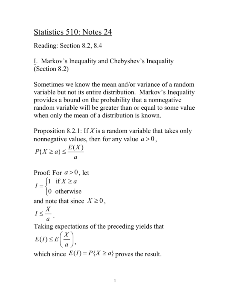
Statistics 510: Notes 24
Reading: Section 8.2, 8.4
I. Markov’s Inequality and Chebyshev’s Inequality
(Section 8.2)
Sometimes we know the mean and/or variance of a random
variable but not its entire distribution. Markov’s Inequality
provides a bound on the probability that a nonnegative
random variable will be greater than or equal to some value
when only the mean of a distribution is known.
Proposition 8.2.1: If X is a random variable that takes only
nonnegative values, then for any value a  0 ,
E( X )
P{ X  a} 
a
Proof: For a  0 , let
1 if X  a
I 
0 otherwise
and note that since X  0 ,
X
I .
a
Taking expectations of the preceding yields that
X
E(I )  E   ,
a
which since E ( I )  P{ X  a} proves the result.
1
As a corollary, we obtain Chebyshev’s Inequality that
provides a bound on the probability of a random variable
departing from its mean by a certain amount if we know the
variance of a random variable.
Proposition 8.2.2: If X is a random variable with finite
2
mean  and variance  , then for any value k  0 ,
P{| X   | k} 
2
k2 .
Proof: Since  X   
2
is a nonnegative random variable,
2
we can apply Markov’s inequality with a  k to obtain
E[( X   ) 2 ]
2
2
P{( X   )  k } 
(1.1)
k2
2
2
But since ( X   )  k if and only if | X   | k ,
Equation (1.1) is equivalent to
E[( X   )2 ]  2
P{| X   | k} 
 2
2
k
k
and the proof is complete.
Example 2: A fair die is tossed 100 times. Let X k denote
the outcome on the kth roll. Use Chebyshev’s Inequality to
get a lower bound for the probability that
X  X1   X100 is between 300 and 400.
2
Example 3: The mean of a list of a million numbers is 10
and the mean of the squares of the numbers is 101. Find an
upper bound on how many of the entries in the list are 14 or
more.
3
As Chebyshev’s inequality is valid for all distributions of
the random variable X, we cannot expect the bound on the
probability to be very close to the actual probability in most
cases.
Consider a normal random variable with mean  and
variance  .
2
Probability
Chebyshev bound
Probability for
X ~ N ( , 2 )
P(| X
P(| X
P (| X
P(| X
  |  )
  | 2 )
  | 3 )
  | 4 )
at most 1
at most 1/ 22  0.25
at most 1/ 32  0.11
at most 1/ 42  0.06
0.3173
0.0465
0.00270
0.000063
As the table shows, Chebsyhev’s bound will be very crude
for a distribution that is approximately normal. Its
importance is that it holds no matter what the shape of the
distribution, so it gives some information about two-sided
tail probabilities whenever the mean and standard deviation
of a distribution can be calculated.
II. Convergence in Probability and the Weak Law of Large
Numbers (Section 8.2)
Limit Theorems:
Limit theorems concern what happens in the limit to the
probability distribution of a random variable Yn in an
infinite sequence of random variables Y1 , Y2 ,
In
4
particular we often consider Yn to be a random variable that
is associated with a random sample of n units, e.g., the
1 n
sample mean Yn  n  X i for a sample X 1 , , X n .
i 1
Although the notion of an infinite sample size is a
theoretical artifact, it can often provide us with some useful
approximations for the finite-sample case.
We will consider three types of convergence for the
probability distribution of a sequence of random variables
Y1 , Y2 , : (i) convergence in probability, (ii) almost sure
convergence and (iii) convergence in distribution.
Convergence in Probability: A sequence of random
variables Y1 , Y2 , converges in probability to a number c
if, for every   0 ,
lim P(| Yn  c |  )  0 or equivalently
n 
lim P(| Yn  c |  )  1 .
n 
Note: The Y1 , Y2 , are typically not independent and
identically distributed randomly variables. The distribution
of Yn changes as the subscript changes, and the convergence
concepts we will discuss describe different ways in which
the distribution of Yn “converges” as the subscript becomes
large.
The weak law of large numbers:
5
Consider a sample of independent and identically
distributed random variables X 1 , , X n . The relationship
X1   X n
X

between the sample mean n
and true
n
mean of the X i ’s, E ( X i )   , is a problem of pivotal
importance in statistics. Typically,  is unknown and we
would like to estimate  based on X n . The weak law of
large numbers says that the sample mean converges in
probability to  .
This means that for a large enough sample size
n , X n will be close to  with high probability.
Theorem 8.2.1. The weak law of large numbers.
Let X 1 , X 2 be a sequence of independent and identically
distributed random variables, each having finite mean
E ( X i )   . Then, for any   0 ,
 X   Xn

P 1
      0 as n   .
n


Proof: We prove the result only under the additional
assumption that the random variables have a finite variance
 2 (it can be proved without this assumption using more
advanced techniques). Because
2
 X1   X n 
 X1   X n  
E
  and Var 

,


n
n



 n
it follows from Chebyshev’s inequality that
6
 X1   X n
 2
P
  2
n

 n
2
Since n 2  0 as n   , the result is proved.
Application of Weak Law of Large Numbers: Monte Carlo
Integration.
Suppose that we wish to calculate
1
I ( f )   f ( x)dx
0
where the integration cannot be done by elementary means
or evaluated using tables of integrals. The most common
approach is to use a numerical method in which the integral
is approximated by a sum; various schemes and computer
packages exist for doing this. Another method, called the
Monte Carlo method, works in the following way.
Generate independent uniform random variables on (0,1) –
that is X 1 , , X n -- and compute
1 n
ˆ
I( f )   f (Xi )
n i 1
By the law of large numbers, for large n, this should be
close to E[ f ( X )], which is simply
1
E[ f ( X )]   f ( x)dx  I ( f ) .
0
This simple scheme can easily be modified in order to
change the range of integration and in other ways.
Compared to the standard numerical methods, it is not
especially efficient in one dimension, but becomes
7
increasingly efficient as the dimensionality of the integral
grows.
As a concrete example, let’s consider the evaluation of
1 1
2
I( f )  
e x / 2 dx
0
2
The integral is that of the standard normal density, which
cannot be evaluated in closed form. From Table 5.1, an
accurate numerical approximation is I ( f )  0.3413 . The
following code for the statistical computing software
package R generates 1000 pseudorandom independent
points the uniform (0,1) distribution and computes
Iˆ( f ) .
> # Generate vector of 1000 independent uniform (0,1)
random variables
> xvector=runif(1000);
> # Approximate I(f) by 1/1000 * sum from i=1 to 1000 of
f(Xi)
> fxvector=(1/(2*pi)^.5)*exp(-xvector^2/2);
> Ihatf=1/1000*sum(fxvector);
> Ihatf
[1] 0.3430698
III. Almost Sure Convergence and the Strong Law of
Large Numbers (Section 8.4)
A type of convergence that is stronger than convergence in
probability is almost sure convergence (sometimes
confusingly known as convergence with probability 1).
8
This type of convergence is similar to pointwise
convergence of a sequence of functions except that the
convergence need not occur on a set with probability 0
(hence the “almost” sure).
Almost sure convergence: A sequence of random variables
Y1 , Y2 , defined on a common sample space converges
almost surely to a number c if, for every   0 ,
P(lim | Yn  c |  )  1 ,
n 
Yn  c)  1
or equivalently, P(lim
n 
Almost sure convergence is a much stronger convergence
concept than convergence in probability and indeed implies
convergence in probability.
Example of a sequence of random variable that converges
in probability but not almost surely:
Consider an experiment with sample space the interval
from 0 to 1 and a uniform probability distribution over the
sample space. We construct a sequence of intervals Wn as
follows: W1 is the interval from 0 to 1/2, W2 is the interval
from 1/2 to 1, W3 is the interval from 0 to 1/3, W4 is the
interval from 1/3 to 2/3, W5 is the interval from 2/3 to 1,
W6 is the interval from 0 to ¼, and so forth. Now for every
point s between 0 and 1, define the value of the random
variable Yn (s) to be -1 if s is in the first half of the interval
9
Wn , 1 if s is in the second half of the interval Wn and 0 if
s is not in the interval Wn
We have E (Yn )  0 for all n . Moreover, for any 0    1 ,
P(| Yn  0 |  ) is the probability that a uniform random
variable is in the interval Wn , which converges in
probability to 0 since the length of the intervals
Wn converges to 0. Thus, the sequence Y1 , Y2 , converges
in probability to 0.
However, no matter how short the intervals Wn become,
every s between 0 and 1 is in some Wn during each left-toright “progression” of these events for increasing n .
Consequently, for each s between 0 and 1, the sequence
Y1 (s), Y2 (s), does not converge and hence Y1 , Y2 , does
not converge almost surely.
The Strong Law of Large Numbers: The strong law of large
numbers states that for a sequence of independent and
identically distributed random variables X 1 , X 2 , the
sample mean converges almost surely to the mean of the
random variables E ( X i )   .
Theorem 8.4.1: Let X1 , X 2 , , be a sequence of
independent and identically distributed random variables,
each having a finite mean   E ( X i ) . Then, with
probability 1,
10
X1 
 Xn
n
  as n   .
What is the strong law of large numbers adding to the weak
law of large numbers?
The weak law of large numbers states that for any specified
*
*
large value n , ( X1   X n* ) / n is likely to be near  .
However, it does not say that ( X1   X n ) / n is bound to
*
stay near  for all values of n larger than n . Thus, it
leaves open the possibly that large values of
| ( X1   X n ) / n   | can occur infinitely often (thought
at infrequent intervals). The strong law shows that this
cannot occur. In particular, it implies that with probability
1, for any positive value  ,
n
Xi


i 1 n
will be greater than  only a finite number of times.
Application of the strong law of large numbers: Consider a
sequence of independent trials of some experiments. Let
E be a fixed event of the experiment and denote by
P ( E ) the probability that the event E occurs on any
particular trial. Letting,
1 if E occurs on the ith trial
Xi  
,
0 if E does not occur on the ith trial
we have by the strong law of large numbers that with
probability 1,
11
X1 
 Xn
 E[ X ]  P( E )
(1.2)
n
Since X 1   X n represents the number of times that the
event E occurs in the first n trials, equation (1.2) is stating
that, with probability 1, the limiting proportion of times
that the event E occurs in repeated, independent trials of
the experiment is just P ( E ) .
The strong law of large numbers is of enormous
importance, because it provides a direct link between the
axioms of probability (Section 2.3) and the frequency
interpretation of probability. If we accept the interpretation
that “with probability 1” means “with certainty,” then we
can say that P ( E ) is the limit of the long-run relative
frequency of times E would occur in repeated, independent
trials of the experiment.
12