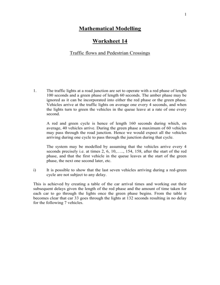
1
Mathematical Modelling
Worksheet 14
Traffic flows and Pedestrian Crossings
1.
The traffic lights at a road junction are set to operate with a red phase of length
100 seconds and a green phase of length 60 seconds. The amber phase may be
ignored as it can be incorporated into either the red phase or the green phase.
Vehicles arrive at the traffic lights on average one every 4 seconds, and when
the lights turn to green the vehicles in the queue leave at a rate of one every
second.
A red and green cycle is hence of length 160 seconds during which, on
average, 40 vehicles arrive. During the green phase a maximum of 60 vehicles
may pass through the road junction. Hence we would expect all the vehicles
arriving during one cycle to pass through the junction during that cycle.
The system may be modelled by assuming that the vehicles arrive every 4
seconds precisely i.e. at times 2, 6, 10,….., 154, 158, after the start of the red
phase, and that the first vehicle in the queue leaves at the start of the green
phase, the next one second later, etc.
i)
It is possible to show that the last seven vehicles arriving during a red-green
cycle are not subject to any delay.
This is achieved by creating a table of the car arrival times and working out their
subsequent delays given the length of the red phase and the amount of time taken for
each car to go through the lights once the green phase begins. From the table it
becomes clear that car 33 goes through the lights at 132 seconds resulting in no delay
for the following 7 vehicles.
2
Car arrival times secs (s)
2
6
10
14
18
22
26
30
34
38
42
46
50
54
58
62
66
70
74
78
82
86
90
94
98
102
106
110
114
118
122
126
130
134
138
142
146
150
154
158
Delay (s)
98
95
92
89
86
83
80
77
74
71
68
65
62
59
56
53
50
47
44
41
38
35
32
29
26
23
20
17
14
11
8
5
2
0
0
0
0
0
0
0
Red Phase
Green
Phase
Car 33 goes through the
lights at 132 seconds
resulting in no delay for the
following 7 vehicles
Red Phase
3
ii)
From the table it is possible to find the average delay per vehicle.
Average Delay per vehicle =
2.
1
1650
Delay (s) 
 41.25 seconds.

40
40
We can consider the traffic light model of question (1) with general values of
the parameters:
rv = length of red phase (seconds).
g v = length of green phase (seconds).
a = time between arrivals of vehicles (seconds).
d = time between departure of vehicles in the queue (seconds).
i)
It is possible to devise a formula to give the average delay per vehicle in terms
of rv , g v , a and d.
Average Delay per vehicle =
N = number of vehicles =
The
1
N
 Delay
rv  g v
a
 Delay can be expressed as the sum of an arithmetic progression:
Sn 
where
1
n A  L 
2
A = first term = a - d
L = last term = rv - 1
n=
rv 1
ad
rv  1 a  d   r  1
v
2a  d 
r  1 1  rv  1 
 v
2  a  d  
Sn 
Average Delay per vehicle =
arv  1  rv  1 
1
2rv  g v   a  d 
4
ii)
If the system is modelled stochastically rather than deterministically, what
effect will this have on the average delay per vehicle?
In this case the car arrival and departure times are random variables.
X = arrival time.
Y = departure time.
 X ~ P0 a 
Y ~ P0 d 
Therefore taking into consideration random variation, if a large number of vehicles
arrive at the traffic lights in a short period of time then the average delay per vehicle
will increase due to the congestion. However if very few cars arrive at the lights over
a short period of time then the average delay per vehicle will decrease because there is
no long standing cue of traffic waiting to go through.
3.
The flow of pedestrians at a road crossing is controlled by a set of traffic lights
that operate on a fixed cycle basis. The red light is shown to pedestrians for
rp seconds, the green light for g p seconds. We can assume that pedestrians
arrive at the rate of one person every b seconds, and that all pedestrians
arriving during the red phase cross the road at the start of the green phase, and
those pedestrians arriving during the green phase cross the road immediately.
From this information we can find a formula for the average delay per
pedestrian.
The formula can be obtained by using a similar method to that used in question (2):
Average Delay per pedestrian =
N = number of pedestrians =
The
1
N
 Delay
rp  g p
b
 Delay can be expressed as the sum of an arithmetic progression:
Sn 
1
n A  L 
2
In this case d will be zero because there is no time between the crossing of
pedestrians.
5
so
A = first term = b
L = last term = rp
n=
Sn 
rp

rp
b

b  rp
2b
rp  rp 
 1  
2 
b
Average Delay per pedestrian =
4.
 rp 
1  
2rp  g p  
b
brp
Pedestrians cross a one-way street at a point P where there are no traffic lights
or other traffic controls. It takes a pedestrian f seconds to cross the road, and
vehicles pass at random such that there is an average of a seconds between the
times when successive vehicles pass point P.
i.e. the number of vehicles that pass point P in one second is a Poisson random
1
variable with mean .
a
i)
It is possible to demonstrate that a deterministic model in which vehicles are
assumed to pass point P at exact intervals of a seconds is inappropriate for
determining the average delay to pedestrians.
Pedestrians can cross if and only if
the times between successive
vehicles passing point P is greater
than the time it takes to cross the
road.
P
a>f
f secs
Car
6
Therefore the deterministic model is inappropriate for determining the delay to
pedestrians because the cars arrive at regular intervals. In reality if a<f then the
pedestrians would never cross the road, which is not a realistic model.
ii)
We can use a stochastic model to determine the average delay to pedestrians in
terms of f and a.
The car interval is a random variable.
1
X ~ P0  
a
N  Waiting time
1
W ~ Ex  
a
P X  f   
f
0

f
0
f


1  at
e dt  1  e a
a


P


1  at
e dt  mean of exponential distribution over f.
a
 a  a  f e

f
a
 A  mean waiting time of 1 vehicle.
AP is the average time one has to wait for 1 car.
AP 2 is the average time one has to wait for 2 cars.
AP 3 is the average time one has to wait for 3 cars.
.
.
.
n
AP is the average time one has to wait for n cars.
This gives
AP  AP 2  AP 3  .....  AP n

 A P  P 2  P 3  .....  P n
This can be written as
the sum of a geometric
series.

7
That is
P
1 P
Therefore the average waiting time for any one person is =
This equation can be re-written in terms of f and a.
f
f

 

a 
a



a

a

f
e
1

e



AP


f
1 P
 

1  1  e a 



a  a  f e

f
a
 ae
e
f
 ae a  a  f e

f
a


f
a




 a  f e
f
a
 f  2a

2f
a
AP
1 P