Checking for Multicollinearity Using SAS
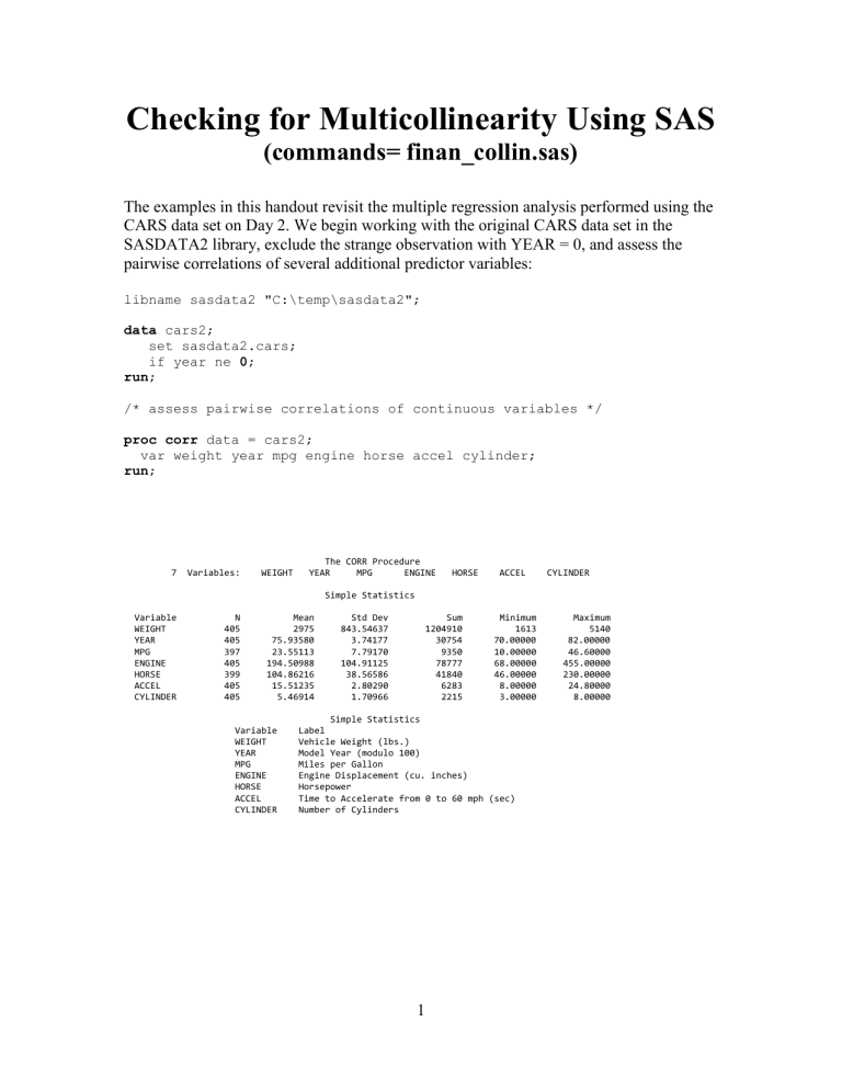
(commands= finan_collin.sas)
The examples in this handout revisit the multiple regression analysis performed using the
CARS data set on Day 2. We begin working with the original CARS data set in the
SASDATA2 library, exclude the strange observation with YEAR = 0, and assess the
pairwise correlations of several additional predictor variables:
libname sasdata2 "C:\temp\sasdata2";
data cars2;
set sasdata2.cars;
if year ne 0;
run;
/* assess pairwise correlations of continuous variables */
proc corr data = cars2;
var weight year mpg engine horse accel cylinder;
run;
7
Variables:
WEIGHT
The CORR Procedure
YEAR
MPG
ENGINE
HORSE
ACCEL
CYLINDER
Simple Statistics
Variable
WEIGHT
YEAR
MPG
ENGINE
HORSE
ACCEL
CYLINDER
N
405
405
397
405
399
405
405
Mean
2975
75.93580
23.55113
194.50988
104.86216
15.51235
5.46914
Variable
WEIGHT
YEAR
MPG
ENGINE
HORSE
ACCEL
CYLINDER
Std Dev
843.54637
3.74177
7.79170
104.91125
38.56586
2.80290
1.70966
Sum
1204910
30754
9350
78777
41840
6283
2215
Minimum
1613
70.00000
10.00000
68.00000
46.00000
8.00000
3.00000
Simple Statistics
Label
Vehicle Weight (lbs.)
Model Year (modulo 100)
Miles per Gallon
Engine Displacement (cu. inches)
Horsepower
Time to Accelerate from 0 to 60 mph (sec)
Number of Cylinders
1
Maximum
5140
82.00000
46.60000
455.00000
230.00000
24.80000
8.00000
Pearson Correlation Coefficients
Prob > |r| under H0: Rho=0
Number of Observations
WEIGHT
Vehicle Weight (lbs.)
WEIGHT
YEAR
MPG
ENGINE
1.00000
-0.30990
<.0001
405
-0.83014
<.0001
397
0.93335
<.0001
405
-0.30990
<.0001
405
1.00000
0.57608
<.0001
397
-0.37932
<.0001
405
-0.83014
<.0001
397
0.57608
<.0001
397
1.00000
-0.80388
<.0001
397
0.93335
<.0001
405
-0.37932
<.0001
405
-0.80388
<.0001
397
1.00000
0.86506
<.0001
399
-0.41946
<.0001
399
-0.77619
<.0001
391
0.89949
<.0001
399
-0.43847
<.0001
405
0.30753
<.0001
405
0.42775
<.0001
397
-0.56226
<.0001
405
0.89482
<.0001
405
-0.35706
<.0001
405
-0.77394
<.0001
397
0.95183
<.0001
405
405
YEAR
Model Year (modulo 100)
MPG
Miles per Gallon
ENGINE
Engine Displacement (cu. inches)
HORSE
Horsepower
ACCEL
Time to Accelerate from 0 to 60 mph (sec)
CYLINDER
Number of Cylinders
405
Pearson Correlation Coefficients
Prob > |r| under H0: Rho=0
Number of Observations
HORSE
397
405
ACCEL
CYLINDER
0.86506
<.0001
399
-0.43847
<.0001
405
0.89482
<.0001
405
YEAR
Model Year (modulo 100)
-0.41946
<.0001
399
0.30753
<.0001
405
-0.35706
<.0001
405
MPG
Miles per Gallon
-0.77619
<.0001
391
0.42775
<.0001
397
-0.77394
<.0001
397
ENGINE
Engine Displacement (cu. inches)
0.89949
<.0001
399
-0.56226
<.0001
405
0.95183
<.0001
405
HORSE
Horsepower
1.00000
-0.70885
<.0001
399
0.84355
<.0001
399
-0.70885
<.0001
399
1.00000
-0.52849
<.0001
405
0.84355
<.0001
399
-0.52849
<.0001
405
WEIGHT
Vehicle Weight (lbs.)
399
ACCEL
Time to Accelerate from 0 to 60 mph (sec)
CYLINDER
Number of Cylinders
405
1.00000
405
We note several extremely large positive and negative correlations, especially of the
ENGINE variable with other possible predictors of MPG. Including several predictors in
a multiple regression model that are highly correlated with each other (multicollinearity)
can have an adverse effect on estimates of regression coefficients (signs may be flipped
entirely) and their significance tests (standard errors tend to be “inflated” and are much
2
larger than they should be, relative to the case where predictors are not correlated). We
consider fitting a regression model using all of these predictors of MPG:
/* fit a regression model using all possible predictors */
proc reg data = cars2;
model mpg = weight year engine horse accel cylinder;
run;quit;
The REG Procedure
Model: MODEL1
Dependent Variable: MPG Miles per Gallon
Number of Observations Read
Number of Observations Used
Number of Observations with Missing Values
405
391
14
Analysis of Variance
DF
Sum of
Squares
Mean
Square
6
384
390
19070
4539.97495
23610
3178.30004
11.82285
Root MSE
Dependent Mean
Coeff Var
3.43844
23.48286
14.64233
Source
Model
Error
Corrected Total
R-Square
Adj R-Sq
F Value
Pr > F
268.83
<.0001
0.8077
0.8047
Parameter Estimates
Variable
Label
Intercept
WEIGHT
YEAR
ENGINE
Intercept
Vehicle Weight (lbs.)
Model Year (modulo 100)
Engine Displacement (cu.
inches)
Horsepower
Time to Accelerate from 0 to
60 mph (sec)
Number of Cylinders
HORSE
ACCEL
CYLINDER
DF
Parameter
Estimate
Standard
Error
t Value
Pr > |t|
1
1
1
1
-14.31877
-0.00680
0.75456
0.00834
4.78551
0.00067085
0.05271
0.00747
-2.99
-10.14
14.31
1.12
0.0029
<.0001
<.0001
0.2647
1
1
-0.00200
0.07502
0.01417
0.10392
-0.14
0.72
0.8877
0.4708
1
-0.34586
0.33376
-1.04
0.3007
Results to note are highlighted in boldface. Despite the fact that ENGINE, HORSE,
ACCEL, and CYLINDER all have significant bivariate correlations with MPG, none of
them appear to be significant predictors of MPG based on the t-tests for their coefficients
in the regression model. What’s happening here? We can assess collinearity diagnostics
using additional options supplied to Proc Reg (vif, tol, and collin):
/* refit model, and request collinearity diagnostics */
proc reg data = cars2;
model mpg = weight year engine horse accel cylinder / vif tol collin;
run;
quit;
3
Parameter Estimates
Variable
Label
Intercept
WEIGHT
YEAR
ENGINE
Intercept
Vehicle Weight (lbs.)
Model Year (modulo 100)
Engine Displacement (cu.
inches)
Horsepower
Time to Accelerate from 0 to
60 mph (sec)
Number of Cylinders
HORSE
ACCEL
CYLINDER
DF
Tolerance
Variance
Inflation
1
1
1
1
.
0.09416
0.80734
0.04964
0
10.62064
1.23864
20.14676
1
1
0.10298
0.36895
9.71021
2.71042
1
0.09382
10.65908
4
Collinearity Diagnostics
Number
Eigenvalue
Condition
Index
1
2
3
4
5
6
7
6.66806
0.28737
0.02426
0.00993
0.00500
0.00459
0.00080065
1.00000
4.81704
16.57992
25.90982
36.53406
38.12909
91.25974
---------------Proportion of Variation--------------Intercept
WEIGHT
YEAR
ENGINE
0.00002873
0.00047589
0.00295
0.00750
0.00298
0.01096
0.97510
0.00015625
0.00053364
0.00647
0.20868
0.53551
0.19390
0.05475
0.00004058
0.00083990
0.00357
0.01533
0.00061181
0.09026
0.88936
0.00022630
0.01247
0.06229
0.00060254
0.76121
0.16068
0.00252
Collinearity Diagnostics
Number
1
2
3
4
5
6
7
---------Proportion of Variation--------HORSE
ACCEL
CYLINDER
0.00026356
0.00388
0.25738
0.07830
0.02938
0.43904
0.19175
0.00023012
0.01143
0.07604
0.15214
0.14182
0.49405
0.12428
0.00018279
0.00119
0.02274
0.30804
0.31621
0.33015
0.02147
The tolerance (requested by the tol option) is the proportion of variance in a given
predictor that is NOT explained by all of the other predictors, while the VIF (or Variance
Inflation Factor) is simply 1 / tolerance. The VIF represents a factor by which the
variance of the estimated coefficient is multiplied due to the multicollinearity in the
model. In other words, the variance of the estimated coefficient for ENGINE is 20 times
larger than it would be if the predictors were orthogonal (i.e., not correlated).
A good “global” check for a multicollinearity problem is to see if the largest condition
index is greater than 30. This is a general rule of thumb, and we definitely see a problem
in this model. Predictors with large proportions of variation for eigenvalues that are very
small (the last three eigenvalues in this case) tend to be highly correlated, and could
possibly be combined rather than considered separately.
At this point, one could arbitrarily choose one of a set of highly correlated predictors to
retain in the model, or possibly combine the correlated predictors into a single variable
(perhaps using a technique known as principal components analysis). We arbitrarily only
include ENGINE as an additional predictor, and refit the model:
/* refit model, including ENGINE only */
proc reg data = cars2;
model mpg = weight year engine /*horse accel cylinder*/ / vif tol
collin;
run;
quit;
Parameter Estimates
Variable
Label
Intercept
WEIGHT
YEAR
ENGINE
Intercept
Vehicle Weight (lbs.)
Model Year (modulo 100)
Engine Displacement (cu.
inches)
DF
Parameter
Estimate
Standard
Error
t Value
Pr > |t|
1
1
1
1
-14.37464
-0.00684
0.76191
0.00148
3.99146
0.00057750
0.05082
0.00479
-3.60
-11.84
14.99
0.31
0.0004
<.0001
<.0001
0.7573
5
6
Parameter Estimates
Variable
Label
Intercept
WEIGHT
YEAR
ENGINE
Intercept
Vehicle Weight (lbs.)
Model Year (modulo 100)
Engine Displacement (cu.
DF
Tolerance
Variance
Inflation
1
1
1
1
.
0.12614
0.85080
0.11994
0
7.92792
1.17536
8.33762
We still see a problem with variance inflation due to the correlation of ENGINE with
WEIGHT (to the point where WEIGHT does not seem to have a significant relationship
with MPG), suggesting that our original model from yesterday would be sufficient. The
largest condition index for this model was about 62.
Be very wary of multicollinearity and its side effects when fitting multiple regression
models using several continuous predictors! Centering variables (see Day 2 handout) can
help, especially when working with interactions between continuous predictors.
Fitting Regression Models Using SAS INSIGHT
1. Type “insight” into the command line dialog box in the SAS window to start SAS
INSIGHT.
2. Select a defined library and a SAS data set to work with.
3. Select Analyze, and then Fit (Y X) to fit a regression model.
4. Select the dependent (Y) variable, and any independent (X) predictor variables
that are defined in the SAS data set. Click OK to fit the model and generate
estimates of the regression coefficients.
5. To investigate additional diagnostic plots after the model has been fitted, use the
Graphs menu. In the case of simple linear regression, confidence curves can be
drawn around the fitted line by using the Curves menu.
6. Additional tables of output (e.g., Collinearity Diagnostics) can be requested using
the Tables menu.
7