Chapter 4
Lecture 10 simultaneous inferences
Set 1
Joint Confidence for the Slope and Intercept
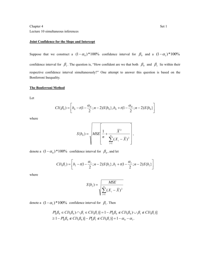
Suppose that we construct a (1   0 ) *100% confidence interval for  0 and a (1  1 ) *100%
confidence interval for
 1 . The question is, “How confident are we that both  0 and  1 lie within their
respective confidence interval simultaneously?” One attempt to answer this question is based on the
Bonferroni Inequality.
The Bonferroni Method
Let




CI (  0 )  b0  t (1  0 ; n  2) S{b0 }, b0  t (1  0 ; n  2) S{b0 }
2
2


where


2
1

X
,
S{b0 )  MSE   n
n
2 
(Xi  X ) 


i 1

denote a (1   0 ) *100% confidence interval for  0 , and let




CI ( 1 )  b1  t (1  1 ; n  2) S{b1 }, b1  t (1  1 ; n  2) S{b1 }
2
2


where
S{b1 ) 
MSE
n
(X
i 1
denote a (1  1 ) *100% confidence interval for
i
 X )2
 1 . Then
P[  0  CI (  0 )  1  CI ( 1 )]  1  P[  0  CI (  0 )  1  CI ( 1 )]
 1  P[  0  CI (  0 )]  P[ 1  CI ( 1 )]  1   0   1 .
Thus, if we want a pair of confidence intervals for  0 and
 1 such that the confidence that both intervals
contain their respective true parameter values is at least (1   ) * 100% , we must pick  0 and
that
 1 such
 0  1   . It is customary to set  0  1   2 . Thus the Bonferroni simultaneous confidence
intervals for  0 and
 1 are
1

X2
b0  t (1   / 4; n  2) MSE  
,
2 
 n  ( X i  X ) 
and
MSE
.
 (X i  X )2
b1  t (1   / 4; n  2)
Example
Recall that in our vehicle weight-MPG example, n  10 , X  33.5 ,
( X
i
 X ) 2  232.5 and
MSE  0.12495 . We will now compute 95% simultaneous confidence intervals for  0 and  1 using
Bonferroni procedure.
95% confidence    0.05 

4
 0.0125  1 

4
 0.9875 . The 98.75th percentile is not given in
Table B.2. However from table B.2 we can get t (.985;8)  2.634 and t (.99;8)  2.896 . After
interpolating, we get t (.9875;8)  2.7695 .
The correct value is t (.9875;8)  2.75152 . We can get this value from SAS by writing the following 5
lines of code.
data;
Obs
t=tinv(.9875,8);
1
t
2.75152
run;
proc print;
run;
Remark: The approximation obtained by interpolation is close enough for practical purpose, but if you want
our results to agree with SAS’s output, we must use the exact percentile.
The standard errors for b0 and b1 are
1
S{b0 }  MSE  
n


X2
  0.78462 ,
2 
(
X

X
)
 i

MSE
S (b1 ) 
n
(X
i 1
i
 0.02318 .
 X)
2
Note: These standard errors can also be obtained directly from the SAS output.
PROC REG DATA=Cars;
MODEL mpg=weight /clb alpha=.05;
RUN;
quit;
Parameter Estimates
Parameter
Standard
Variable
DF
Estimate
Error
t Value
Pr > |t|
Intercept
1
23.65677
0.78462
30.15
<.0001
21.84745
25.46610
weight
1
-0.19871
0.02318
-8.57
<.0001
-0.25217
-0.14525
Thus, the 95% Bonferroni confidence intervals for  0 and
95% Confidence Limits
 1 are
23.65677  2.75152 * .78462  23.65677  2.15890 ,
 0.19871  2.75152 * .02318  0.19871  0.06378
respectively.
That is, we are 95% confident that both
21.4979   0  25.8157
&
 0.262550  1  0.13492 .
Notice that the 95% Bonferroni intervals are slightly larger than the individual 95% confidence intervals.
Note: The 95% Bonferroni confidence intervals for  0 and
for  0 and
 1 can be obtained by calculating 97.5% CI
 1 respectively.
/* compute 95% simultaneous CLB using Bonferroni procedure*/
proc reg data=Cars;
model mpg=weight/clb alpha=.025;
run;
Simultaneous Estimation of the mean value of Y for multiple values of X
Often the mean value of response variable Y needs to be estimated for more than one value of X. There are
two approaches to this problem, the working-Hotelling procedure and the Bonferroni method.
The working-Hotelling Method
This procedure has already been introduced in chapter 2. Suppose that we want to obtain simultaneous
(1   )  100% confidence intervals for E (Yh ) for several values of X h , say h  h1 , h2 ,, hg . For
each index h, the (1   )  100% Working-Hotelling simultaneous (1   )  100% confidence interval
for E (Yh ) is
( X h  X )2
1
ˆ
, with W  2  F (1   ;2, n  2) .
Yh  W MSE

n  (X i  X )2
The Bonferroni Method
We intend to obtain simultaneous confidence intervals for E (Yh ) at g different values of X h
( h  h1 , h2 , , hg ). Thus the Bonferroni simultaneous (1   )  100% confidence intervals are
( X h  X )2
1
ˆ
Yh  B( , g ) MSE

, with B( , g )  t (1   2 g ; n  2) .
n  ( X i  X )2
Comparison of the two approaches
1. The main difference in the two methods is that the Working-Hotelling value W , depends on
confidence level) only, while B( , g ) depends on both
 (the
 and g .
2. Consequently, if g is reasonably large, the Bonferroni method will produce wider intervals than the
Working-Hotelling approach. When g is small, the Bonferroni method may produce tighter confidence
intervals than Working-Hotelling, but this is not necessary always the case.
3. Since that the Working-Hotelling method does not depend on the # of X-values involved, it can be used to
construct the confidence band for the whole least square regression line as was discussed in Chapter 2.
Example
In our vehicle Weight-MPG example, suppose that we want 95% simultaneous confidence intervals for the
mean MPG for vehicles that weight 3000, 3300 and 3500 pounds respectively. Recall that the least-square
regression line for the data is Yˆh  23.6568  0.19871X h . So,
When X h  30 , Yˆh  23.6568  0.19871 30  17.6955 ,
When X h  33 , Yh  23.6568  0.19871 33  17.0994 ,
When X h  35 , Yˆh  23.6568  0.19871 35  16.7019 .
Also,
(X h  X )2
1
,
S{Yˆh }  MSE

n  (X i  X )2
So,
When X h  30 , S{Yˆh }  .12495
1 (30  33.5) 2

 0.13813 ,
10
232.5
When X h  33 , S{Yˆh }  0.11238 ,
When X h  35 , S{Yˆh }  0.11707
To compute the 95% Working-Hotelling intervals, not that since W 
2  F (1   ;2, n  2) ,
W (0.05)  2  F (0.95;2,8)  2  4.45896  2.98629 , which can be calculated by the following
SAS code.
data;
proc print;
F=finv(.95,2,8);
run;
W=sqrt(2*F);
Obs
F
W
1
4.45897
2.98629
run;
Thus, when X h  30 , the 95% Working-Hotelling limits are
17.6955  (2.98629  .13813)  17.6955  .41248 , i.e., 17.2830  E (Yh )  18.1080 .
Similarly, at X h  33 , 16.7638  E (Yh )  17.4350 . At X h  35 , 16.3523  E (Yh )  17.0515 .
That is, with 95% Working-Hotelling procedure, we can be 95 % confident that the mean MPG
are all between
17.2830MPG and 18.1080MPG, when the vehicles weight 3000 pounds.
16.7638MPG and 17.4350MPG, when the vehicles weight 3300 pounds.
16.3523MPG and 17.0515MPG, when the vehicles weight 3500 pounds.
To compute the 95% Bonferroni confidence intervals, note that for g  3 and   0.05 , we
have 1   /( 2 g )  1  .05 / 6  0.991667 , and B(.05,3)  t (.991667,8)  3.10579 , which is
obtained from the following SAS code:
data;
proc print;
Obs
t=tinv(.991667,8);
run;
1
t
3.01579
run;
Thus, when X h  30 , limits are 17.6955  (3.01579  .13813)  17.6955  .4165 , i.e., That is,
when X h  30 , 17.2790  E (Yh )  18.1120 . Similarly, at X h  33 ,
16.7605  E (Yh )  17.4383 And at X h  35 , 16.3489  E (Yh )  17.0550 .
So, with 95% Bonferroni procedure, we can be 95% confident that the mean MPG are all between
17.2790MPG and 18.1120MPG, when the vehicles weight 3000 pounds.
16.7605MPG and 17.4383MPG, when the vehicles weight 3300 pounds.
16.3489MPG and 17.0550MPG, when the vehicles weight 3500 pounds.
1. The Bonferroni 95% simultaneous confidence limits are slightly larger than the Working-Hotelling
intervals in this example, even though g  3 is rather small.
2. Both the Bonferroni and Working-Hotelling intervals are larger than the ordinary 95%
confidence intervals for the mean response.
/* compute 95% simultaneous CI for mean response at 3 different
levels of predictor variable using Bonferroni procedue*/
data new;
proc reg data=Cars;
INPUT weight mpg;
model mpg=weight/alpha=.0167;
DATALINES;
output out=cars2 p=PredMPG lclm=lower_CI
30 .
stdp=std_EstimatedMean uclm=upper_CI;
33 .
run;
35 .
proc print data=Cars2;
;
run;
run;
data Cars;
set Cars new;
run;
Simultaneous prediction Intervals for New values of Y Given Multiple Values of X
Again there are two methods for computing simultaneous prediction intervals for new responses
corresponding to various values of the predictor variable X. They are the Scheffe method (of which the
Working-hotelling procedure is a special case) and the Bonferroni method.
Recall from Chapter 2 that the standard error for predicting new values of Yh (new) given X h is
S h {Pr ed }  MSE 1 
( X h  X )2
1
.

n  ( X i  X )2
The Scheffe Method
Using the Scheffe method, (1   )  100% simultaneous prediction intervals for Yh (new) are given by
Yˆh  S ( , g )S h {Pr ed} , with S ( , g )  g  F (1   ; g , n  2) .
Note: When g  2 , S ( , g )  W ( ) .
The Bonferroni Method
Using the Bonferroni method, (1   )  100% simultaneous prediction intervals for Yh (new) are
given by



; n  2  .
Yˆh  B( , g )S h {Pr ed} , with B( , g )  t 1 
 2g

Remark:
1. The difference Between CI and PI using Bonferroni method comes about because S{Yˆh }  S h {Pr ed} .
2. With the working-Hotelling modification of the Scheffe method, the standard error is always multiplied by
S ( ,2)  W ( ) when finding confidence intervals for the mean responses whereas when computing
prediction intervals for new responses, the Scheffe procedure depends on the number of X-values for which
the new responses will be predicted.
Example
In our Weight-MPG example, suppose that we want 95% simultaneous prediction intervals for
Yh j (new)
j  1,2,3 , where X h1  30 , X h1  33 and X h1  35 .
As we already know, Yˆh1  17.6955 , Yˆh2  17.0994 and Yˆh3  16.7019 .
Also, B(.05,3)  t (.991667,8)  3.10579 .
1 (30  33.5) 2

 0.3795 ,
Finally, When X h  30 , S h {Pr ed }  .12495 1 
10
232.5
When X h  33 , S h {Pr ed }  0.3709 ,
When X h  35 , S h {Pr ed }  0.3724 .
The 95% simultaneous Bonferroni prediction limits for X  X h ( h  h1 , h2 , h3 ) are given by
Yˆh  B(0.05,3)S h {Pr ed} .
Thus,
16.5510  Yh ( new)  18.8400 at X h  30 ,
15.9808  Yh ( new)  18.2179 at X h  33 ,
15.5792  Yh ( new)  17.8249 at X h  35 .
So with 95% Bonferroni procedure, we can be 95% confident that actual MPG will all be
between
16.5510MPG and 18.8400MPG, when the vehicles weight 3000 pounds.
15.9808MPG and 18.2179MPG, when the vehicles weight 3300 pounds.
15.5792MPG and 17.8249MPG, when the vehicles weight 3500 pounds.
When g  3 , the Scheffe value is S (0.05,3)  3  F (0.95;3,8)  3  4.0662  3.493 , which
can be calculated from the following SAS code:
data;
proc print;
F=finv(.95,3,8);
run;
W=sqrt(3*F);
Obs
F
W
1
4.06618
3.49264
run;
So, 17.6955  3.493  0.3795  Yh ( new)  17.6955  3.493  0.3795 when X h  30 ,
15.8040  Yh ( new)  18.3948 at X h  33 and 15.4012  Yh ( new)  18.0026 at X h  35 .
Thus with 95% Scheffe procedure, we can be 95% confident that the actual MPG will all be
between
16.3700MPG and 19.0210MPG, when the vehicles weight 3000 pounds.
15.8040MPG and 18.3948MPG, when the vehicles weight 3300 pounds.
15.4012MPG and 18.0026MPG, when the vehicles weight 3500 pounds.
Remark: This time the Bonferroni procedure gives the shorter intervals.
Conclusion:
In general, I prefer the Working-Hotelling modification of the Scheffe procedure to compute simultaneous
confidence intervals for the mean responses given multiple values of the predictor variable because the
Working-Hotelling multiplier,
W  2  F (1   ;2, n  2) ,
dose not depend on the # of X-values used. This is why this method can be used to construct confidence
band for the whole regression line.
However, for simultaneously predicting new responses for more than one value of the predictor variable, I
prefer the Bonferroni approach because it tends to give shorter intervals than Scheffe’s method.
/* Compute 95% simultaneous PI for new individual response at 3 different
levels of predictor variable using Bonferroni procedue*/
proc reg data=Cars;
model mpg=weight/alpha=.0167;
output out=cars3 p=PredMPG Lcl=Lower_PI stdI=std_prediction UCL=Upper_PI;
run;
proc print data=Cars3;
run;