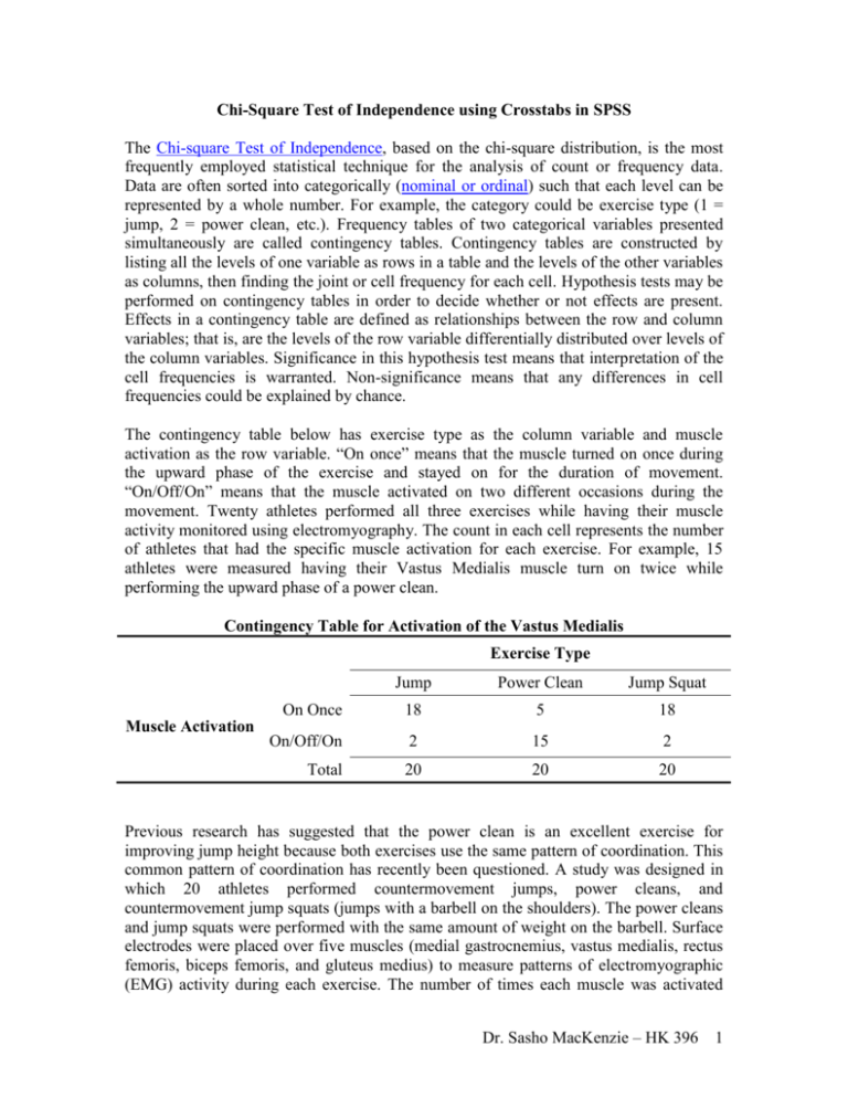
Chi-Square Test of Independence using Crosstabs in SPSS
The Chi-square Test of Independence, based on the chi-square distribution, is the most
frequently employed statistical technique for the analysis of count or frequency data.
Data are often sorted into categorically (nominal or ordinal) such that each level can be
represented by a whole number. For example, the category could be exercise type (1 =
jump, 2 = power clean, etc.). Frequency tables of two categorical variables presented
simultaneously are called contingency tables. Contingency tables are constructed by
listing all the levels of one variable as rows in a table and the levels of the other variables
as columns, then finding the joint or cell frequency for each cell. Hypothesis tests may be
performed on contingency tables in order to decide whether or not effects are present.
Effects in a contingency table are defined as relationships between the row and column
variables; that is, are the levels of the row variable differentially distributed over levels of
the column variables. Significance in this hypothesis test means that interpretation of the
cell frequencies is warranted. Non-significance means that any differences in cell
frequencies could be explained by chance.
The contingency table below has exercise type as the column variable and muscle
activation as the row variable. “On once” means that the muscle turned on once during
the upward phase of the exercise and stayed on for the duration of movement.
“On/Off/On” means that the muscle activated on two different occasions during the
movement. Twenty athletes performed all three exercises while having their muscle
activity monitored using electromyography. The count in each cell represents the number
of athletes that had the specific muscle activation for each exercise. For example, 15
athletes were measured having their Vastus Medialis muscle turn on twice while
performing the upward phase of a power clean.
Contingency Table for Activation of the Vastus Medialis
Exercise Type
Muscle Activation
Jump
Power Clean
Jump Squat
On Once
18
5
18
On/Off/On
2
15
2
Total
20
20
20
Previous research has suggested that the power clean is an excellent exercise for
improving jump height because both exercises use the same pattern of coordination. This
common pattern of coordination has recently been questioned. A study was designed in
which 20 athletes performed countermovement jumps, power cleans, and
countermovement jump squats (jumps with a barbell on the shoulders). The power cleans
and jump squats were performed with the same amount of weight on the barbell. Surface
electrodes were placed over five muscles (medial gastrocnemius, vastus medialis, rectus
femoris, biceps femoris, and gluteus medius) to measure patterns of electromyographic
(EMG) activity during each exercise. The number of times each muscle was activated
Dr. Sasho MacKenzie – HK 396
1
was determined from the EMG signal. The researcher hypothesized that the knee flexors
(vastus medialis and rectus femoris) would show different patterns of activation due to
the power clean’s characteristic 2nd knee flexion during the upward phase. The knees flex
once during the downward phase of the power clean, and then again about 2/3 into the
upward movement. This is not seen during a jump.
The crosstabulation table is the basic technique for examining the relationship between
two categorical variables (muscle activation pattern and exercise), possibly controlling
for additional layering variables (individual muscles). The Crosstabs procedure in SPSS
offers tests of independence. Use the Crosstabs procedure to test the hypothesis that the
patterns of muscle activation are consistent across the different exercises depending on
the muscle investigated.
Open SPSS from the Webfx folder on the desktop, and then open the file Chi Square
EMG Sasho.sav. The data must be set-up in a particular manner in order to use Crosstabs
and to perform a Chi Square Test of Independence (Figure 1). The Subject column
identifies the subject (1 to 20). The Exercise column identifies the type of exercise (1 =
Jump, 2 = Power Clean, 3 = Jump Squat). The Muscle column identifies the specific
muscle (1 = gastroc, 2 = vastus med, 3 = rectus, 4 = biceps fem., 5 = gluteus). The
Activation column represents the number of times the muscle turned on. For example, the
first row indicates that Subject 1, while performing exercise 1 (Jump), had muscle
1(gastroc) turn on 2 times. There are, 20 subjects x 3 exercises x 5 muscles = 300
different activation counts, so there are 300 rows in the file.
Figure 1
Dr. Sasho MacKenzie – HK 396
2
To perform the Chi Square Test of Independence, you need to click on the Analyze ->
Descriptive Statistics -> Crosstabs, as in Figure 2.
Figure 2
After this, the Crosstabs dialog box will appear (Figure 3). In this box, you'll be able to
select the categorical variables to be cross-tabulated. Activation is the row variable and
Exercise is the column variable, while Muscle is the “Layer” variable. By selecting a
layer variable, SPSS will perform a separate Chi Square test for each of the 5 muscles.
This is important since only some muscles may demonstrate different patterns of
activation depending on the exercise, while other muscles may have the same pattern of
activation for each exercise. Check, Display clustered bar charts, and then click
Statistics.
In the Crosstabs: Statistics box (Figure 4), check Chi-square and Phi and Cramer’s V,
then hit Continue. From the original Crosstabs box, select Cells.
In the Crosstabs: Cell Display box, make the selection shown in Figure 5 below and hit
continue. From the original Crosstabs box, select Exact.
In the Exact Tests box (Figure 6), select Exact, and then hit Continue. From the
Crosstabs box hit OK to run the analysis.
Dr. Sasho MacKenzie – HK 396
3
Figure 3
Figure 4
Dr. Sasho MacKenzie – HK 396
4
Figure 5
Figure 6
The observed and expected frequencies are shown for three muscles in the SPSS output
in Figure 7 below. By comparing the cells highlighted in turquoise for the knee flexor
muscles, you can see that the Clean has a much higher count for the On/Off/On scenario.
For the Vastus Medialis, 15 of the subjects had a double activation for the Clean, while
only 2 should a double activation for the Jump and Jump Squat. While this “looks”
different, this qualitative assessment needs to be confirmed with a statistical test.
Dr. Sasho MacKenzie – HK 396
5
Number of Activa tions * Type of Exerice * Muscle Crosstabulation
Ty pe of Ex erice
Jump
Clean
Jump Squat
Total
Number of On onc e
Count
16
16
17
49
Ac tivat ions
Ex pec ted Count
16.3
16.3
16.3
49.0
Residual
-.3
-.3
.7
St d. Residual
-.1
-.1
.2
Adjust ed Residual
-.2
-.2
.5
On/Off/On Count
4
4
3
11
Ex pec ted Count
3.7
3.7
3.7
11.0
Residual
.3
.3
-.7
St d. Residual
.2
.2
-.3
Adjust ed Residual
.2
.2
-.5
Total
Count
20
20
20
60
Ex pec ted Count
20.0
20.0
20.0
60.0
Vastus Medialus Number of On onc e
Count
18
5
18
41
Ac tivat ions
Ex pec ted Count
13.7
13.7
13.7
41.0
Residual
4.3
-8. 7
4.3
St d. Residual
1.2
-2. 3
1.2
Adjust ed Residual
2.6
-5. 1
2.6
On/Off/On Count
2
15
2
19
Ex pec ted Count
6.3
6.3
6.3
19.0
Residual
-4. 3
8.7
-4. 3
St d. Residual
-1. 7
3.4
-1. 7
Adjust ed Residual
-2. 6
5.1
-2. 6
Total
Count
20
20
20
60
Ex pec ted Count
20.0
20.0
20.0
60.0
Rectus Femoris Number of On onc e
Count
15
5
17
37
Ac tivat ions
Ex pec ted Count
12.3
12.3
12.3
37.0
Residual
2.7
-7. 3
4.7
St d. Residual
.8
-2. 1
1.3
Adjust ed Residual
1.5
-4. 1
2.6
On/Off/On Count
5
15
3
23
Ex pec ted Count
7.7
7.7
7.7
23.0
Residual
-2. 7
7.3
-4. 7
St d. Residual
-1. 0
2.6
-1. 7
Adjust ed Residual
-1. 5
4.1
-2. 6
Total
Count
20
20
20
60
Ex pec ted Count
20.0
20.0
20.0
60.0
Bic eps Femoris
Number of On onc e
Count
12
17
15
44
Figure
7
Ac tivat ions
Ex pec ted Count
14.7
14.7
14.7
44.0
Residual
-2. 7
2.3
.3
St d. Residual
-.7
.6
.1
Adjust
ed Residual
The table below (Figure 8) shows the
results
of the Chi-square
test
As
-1. 7
1.4 of Independence.
.2
On/Off/On
Count
8 can see
3 that both5 the Vastus
16
usual a p-value < .05 indicates
statistical
significance. We
pec ted Count
5.3
5.3
Medialis and Rectus Femoris haveExsignificant
Chi-square
values,
which 5.3
confirms16.0
our
Residual
2.7
-2. 3
-.3
visual inspection of the cell counts in
the figure above. Note
the -1.
highlighted
points a) and
St d. Residual
1.2
0
-.1
i) below the table, you will see thatAdjust
we’ve
violated
an
assumption
of
the
Chi-square
test.
ed Residual
1.7
-1. 4
-.2
Total an expected cell
Countcount less than 5.
20 When this
20
20 we should
60
No cell should have
happens
pec ted
Count
20.0 However,
60.0
report the Fisher Exact Test and notExthe
Chi-square
test20.0
(Warner,20.0
2008, p.334).
Medius
onc e
Count
19
18
17
theGluteus
expected
cellNumber
countsof forOnthe
Vastus
Medialis and Rectus
Femoris
are greater
than 5,54so
Ac tivat ions
Ex pec ted Count
18.0
18.0
18.0
54.0
we can report on the Chi-square statistic
for these muscles.
Residual
1.0
.0
-1. 0
St d. Residual
.2
.0
-.2
Adjust ed Residual
.9
.0
-.9
On/Off/On Count
1
2
3
6
Ex pec ted Count
2.0
2.0
2.0
6.0
Residual
-1. 0Sasho MacKenzie
.0
1.0
Dr.
– HK 396 6
St d. Residual
-.7
.0
.7
Adjust ed Residual
-.9
.0
.9
Total
Count
20
20
20
60
Muscle
Gastrocnemius
Chi-Square Tests
Muscle
Gastrocnemius
Vastus Medialus
Rectus Femoris
Biceps Femoris
Gluteus Medius
Pearson Chi-Square
Likelihood Ratio
Fis her's Exact Test
Linear-by-Linear
As sociation
N of Valid Cases
Pearson Chi-Square
Likelihood Ratio
Fis her's Exact Test
Linear-by-Linear
As sociation
N of Valid Cases
Pearson Chi-Square
Likelihood Ratio
Fis her's Exact Test
Linear-by-Linear
As sociation
N of Valid Cases
Pearson Chi-Square
Likelihood Ratio
Fis her's Exact Test
Linear-by-Linear
As sociation
N of Valid Cases
Pearson Chi-Square
Likelihood Ratio
Fis her's Exact Test
Linear-by-Linear
As sociation
N of Valid Cases
Exact Sig.
(2-sided)
1.000
1.000
1.000
Exact Sig.
(1-sided)
Point
Probability
2
2
As ymp. Sig.
(2-sided)
.895
.892
1
.685
.841
.420
.147
2
2
.000
.000
.000002
.000
.000002
1
1.000
1.000
.567
.133
2
2
.000
.000
.000154
.000
.000221
.416
1
.519
.629
.315
.104
60
3.239g
3.268
3.110
2
2
.198
.195
.237
.237
.237
1.131
1
.287
.376
.188
.081
60
1.111i
1.158
1.142
2
2
.574
.561
.863
.863
.863
1
.296
.439
.220
.123
Value
.223a
.229
.329
b
.164
60
26.033 c
26.420
24.715
d
.000
60
17.485 e
17.986
17.025
f
h
j
1.093
df
60
a. 3 cells (50.0%) have expected count less than 5. The minimum expected count is 3.67.
b. The standardized statistic is -.405.
c. 0 cells (.0%) have expected count less than 5. The minimum expected count is 6.33.
d. The standardized statistic is .000.
e. 0 cells (.0%) have expected count less than 5. The minimum expected count is 7.67.
f. The standardized statistic is -.645.
g. 0 cells (.0%) have expected count less than 5. The minimum expected count is 5.33.
h. The standardized statistic is -1.064.
i. 3 cells (50.0%) have expected count less than 5. The minimum expected count is 2.00.
j. The standardized statistic is 1.045.
Figure 8
The significant Chi-square results indicate that there is a reliable relationship between the
variables, but it doesn’t indicate the strength of the relationship, which is referred to as
the effect size. Phi is the most common effect size statistic reported when interpreting the
results of a Chi-square analysis and has the same range as Cohen’s d. The table below
(Figure 9) indicates that the relationship is strong for both the Vastus Medialis and Rectus
Femoris.
Dr. Sasho MacKenzie – HK 396
7
Symm etri c Me asures
Muscle
Gastrocnemius
Nominal by
Nominal
Phi
Cramer's V
Vastus Medialus
N of V alid Cases
Nominal by
Nominal
Phi
Cramer's V
Rectus Femoris
N of V alid Cases
Nominal by
Nominal
Phi
Cramer's V
Biceps Femoris
N of V alid Cases
Nominal by
Nominal
Phi
Cramer's V
Gluteus Medius
N of V alid Cases
Nominal by
Nominal
Phi
Cramer's V
N of V alid Cases
Value
.061
.061
60
.659
.659
60
.540
.540
60
.232
.232
60
.136
.136
60
Approx . Sig. Ex act Sig.
.895
1.000
.895
1.000
.000
.000
.000
.000
.000
.000
.000
.000
.198
.198
.237
.237
.574
.574
.863
.863
a. Not as suming the null hypothes is.
b. Us ing the asymptotic s tandard error ass uming the null hypot hesis.
Figure 9
Now that we know there is a significant, and meaningful, relationship, we have to
perform a post hoc analysis to determine where the differences exist. This is similar to a
Tukey or Scheffe test following the initial F-test with an ANOVA. We will compare the
standardized residuals as suggested by Beasley and Schumaker (1995). This was found to
maintain Type I error at a satisfactory level by MacDonald and Gardner (2000). The
standardized residuals are found in Figure 7 above. Those standardized residuals which
are greater than 1.96 (or less than -1.96) indicate those exercises that contributed to the
significant Chi-square finding. Not surprisingly, we can see that the standardized
residuals for the Clean are greater than 1.96. Therefore we can conclude that the pattern
of muscle activation during the Clean was different from both the Jump and Jump Squat,
but that the pattern between the Jump and Jump Squat was not different.
These results would be written up as follows for the Vastus Medialis:
Of the 20 participants, 15 demonstrated a double activation pattern of the Vastus Medialis
during the upward phase of the power clean, while only 2 participants showed a double
activation pattern for both the jump and jump squat. This was a statistically significant
association: 2 (2) = 26.03, p < .001, with a strong effect size ( = .659). Post-hoc tests,
using standardized residuals, indicated that the pattern of muscle activation during the
Clean was different from both the Jump and Jump Squat, but that the pattern between the
Jump and Jump Squat was not different.
Dr. Sasho MacKenzie – HK 396
8