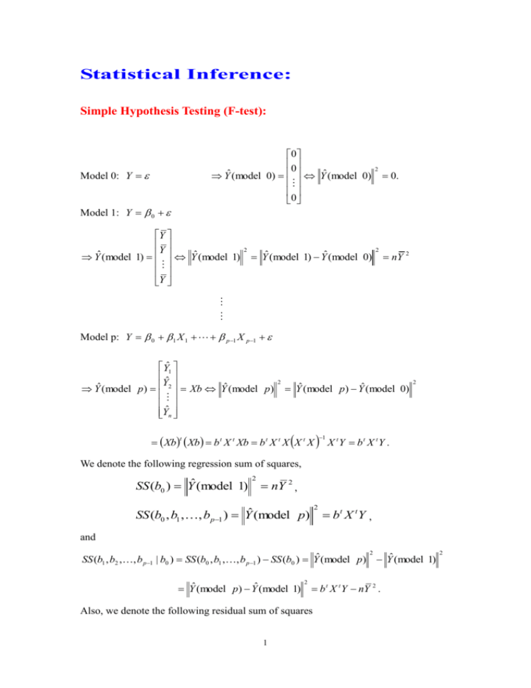
Statistical Inference:
Simple Hypothesis Testing (F-test):
0 
0 
 Yˆ (model 0)     Yˆ (model 0)

 
0 
Model 0: Y  
Model 1: Y   0  
Y 
 
Y
ˆ
 Y (model 1)     Yˆ (model 1)

 
Y 
2
 Yˆ (model 1)  Yˆ (model 0)
2
 0.
2
 nY 2


Model p: Y   0   1 X 1     p 1 X p 1  
Yˆ1 
ˆ 
Y
 Yˆ (model p )   2   Xb  Yˆ (model p )

 
ˆ
Yn 
2
 Yˆ (model p )  Yˆ (model 0)

  Xb  Xb  b t X t Xb  b t X t X X t X
t

1
2
X tY  bt X tY .
We denote the following regression sum of squares,
SS (b0 )  Yˆ (model 1)
2
 nY 2 ,
2
SS (b0 , b1 , , bp1 )  Yˆ (model p)
 bt X t Y ,
and
2
SS (b1 , b2 ,, b p 1 | b0 )  SS (b0 , b1 ,, b p 1 )  SS (b0 )  Yˆ (model p)  Yˆ (model 1)
 Yˆ (model p)  Yˆ (model 1)
2
 b t X t Y  nY 2 .
Also, we denote the following residual sum of squares
1
2
RSS (model p)  Y  Yˆ (model p)


2
 Y  Xb
2
 Y  Xb Y  Xb
t
 Y t  b t X t Y  Xb  Y t Y  2b t X t Y  b t X t Xb

 Y t Y  2b t X t Y  b t X t X X t X
 Y
2

1
X t Y  Y t Y  2b t X t Y  b t X t Y  Y t Y  b t X t Y
2
 Yˆ (m o d epl)
Yˆi
0
Y
(model 0)
(model 1)
SS (b0 )
Yi
(model p)
(data)
SS (b1 ,  , b p1 | b0 )
R S S(m o d epl)
n
Y
2
i
i 1
We have the following fundamental equation:
Fundamental Equation:
n
Y  Yˆ (model 0)   Yi 2
2
i 1
2
2
 Y  Yˆ (model p)  Yˆ (model p)  Yˆ (model 1)  Yˆ (model 1)  Yˆ (model 0)
2
 RSS (model p)  SS (b1 ,, b p 1 | b0 )  SS (b0 )

(the distance between the data and model 0) =
(the distance between the data and model p) +
(the distance between model p and model 1) +
(the distance between model 1 and model 0)
The anova table associated with the fundamental equation is
Source
RSS (model p)
SS (b0 , b1 ,b p 1 )
Total
df
SS
n-p
Y Y b X Y
SS (b0 )
1
nY
SS (b1 ,, bP1 | b0 )
p-1
b t X t Y  nY 2
n
Y
t
t
2
MS
MS (residual p )
2
n
  Yi 2
i 1
2
t
MS (b0 ,, b p 1 )
Note:
RSS (mod el. p) Y t Y  b t X t Y
MS (residual . p) 

n p
n p
MS (b0 , b1 ,, bp1 ) 
SS (b0 , b1 ,, bp1 )
p
bt X tY

p
,
,
and
MS (b1 , , bp1 | b0 ) 
SS (b1 , , bp1 | b0 )
p 1
bt X tY  nY 2

p 1
Simple Hypothesis Testing:
(i) H 0 :  0   1     p 1  0
To test the above hypothesis, the following F statistic can be used,
bt X tY
MS (b0 , b1 , , bp1 )
p
F
 t
Y Y  bt X tY
MS (residual p)
n p


Intuitively, MS (b0 ,, b p 1 ) measures the difference between model p and model 0
while MS (residual p ) is the estimate of the variance  2 of the random error. Thus,
large F value implies the difference between model p and model 0 is large as the
random variation reflected by the mean residual sum of square MS (residual p ) is
taken into account. That is, at least some of  0 ,  1 ,,  p 1 are so significant such
that the difference between model p and model 0 (no parameter) is apparent.
Therefore, the F value can provide important information about if
H 0 :  0   1     p 1  0 . Next question is to ask how large value of F can be
considered to be large? By the distribution theory and the 3 assumptions about the
random errors  i , F ~ F p ,n  p as H 0 :  0   1     p 1  0
3
is true, where
F p ,n  p is the F distribution with degrees of freedom p and n-p, respectively.
(ii) H 0 :  1   2     p 1  0
To test the above hypothesis, the following F statistic can be used,
b X Y  nY 
t
F
MS (b1 , b2 , , b p1 | b0 )
MS (residual p)

t
2
p 1
Y Y  bt X tY
n p

t

Large F value implies the difference between model p and model 1 is large as the
random variation reflected by the mean residual sum of square MS (residual p ) is
taken into account. That is, at least some of  1 ,  2 ,,  p 1 are so significant such
that the difference between model p and model 1 (only one parameter  0 ) is apparent.
F ~ F p 1,n  p as H 0 :  1   2     p 1  0
is true, where F p 1,n  p is the F
distribution with degrees of freedom p-1 and n-p, respectively.
Testing for Several Parameters Being 0: H 0 :  q   q 1     p 1  0
To test the above hypothesis, we need to derive some basic quantities for model q
(q<p), model q: Y   0   1 X 1     q 1 X q 1   . Let
1 X 11
1 X
21

X 



1 X n1
 X 1q 1 
 X 2 q 1 
. Then, the least square estimate for model q is

 

 X nq1 
 b0* 
 * 
b1 

* t
* 1
* t

b  (( X ) X ) ( X ) Y 
  
 * .
bq 1 
4
Then, the fitted value for model q
Yˆ (model q)  X *b*
and the distance between model q and model 0 is
2
SS (b0 , b1 , , bq1 )  Yˆ (model q)  Yˆ (model 0)  (b* )t ( X * )t Y .
Thus, the distance between model p and model q is
Yˆ ( model p )  Yˆ (model q )

2
 
 Yˆ ( model p )  0  Yˆ (model q )  0
 Yˆ (model p )  0
2

2
2
 Yˆ (model q )  0
 SS (b0 , b1 ,, b p 1 )  SS (b0 , b1 , , bq 1 )
 b t X t Y  (b  ) t ( X  ) t Y
 SS (bq , bq 1 ,, b p 1 | b0 , b1 , , bq 1 )
Also,
Yˆ ( model p )  Yˆ ( model q )

2
 
 Y  Yˆ ( model q )  Y  Yˆ ( model p )
 Y  Yˆ ( model q )
2

 Y  Yˆ ( model p )
 RSS ( model q )  RSS ( model p )

 (Y t Y  (b  ) t ( X  ) t Y )  Y t Y  b t X t Y
 b t X t Y  (b  ) t ( X  ) t Y
To test the above hypothesis, the following F statistic can be used,
5

2
2
b X Y  (b ) ( X
t
F
MS (bq , bq1 , , b p1 | b0 , b1 , , bq1 )
MS (residial p)

t
* t
pq
Y Y  bt X tY
n p

t
* t
)Y


,
where
MS (bq , bq 1 ,, b p 1 | b0 , b1 ,, bq 1 ) 
SS (bq , bq 1 ,, b p 1 | b0 , b1 ,, bq 1 )
.
pq
Large F value implies the difference between model p and model q is large as the
random variation reflected by the mean residual sum of square MS (residual p ) is
taken into account. That is, at least some of  q ,  q 1 ,,  p 1 are so significant such
that the difference between model p and model q is apparent. F ~ F p  q ,n  p as
H 0 :  q   q 1     p 1  0 is true, where F p  q ,n  p is the F distribution with
degrees of freedom p-q and n-p, respectively.
Note:
SS (bq , bq 1 ,, b p 1 | b0 , b1 ,, bq 1 )  SS (b0 , b1 ,, b p 1 )  SS (b0 , b1 ,, bq 1 )

 
 SS (b0 , b1 ,, b p 1 )  SS (b0 )  SS (b0 , b1 ,, bq 1 )  SS (b0 )

 SS (b1 ,, b p 1 | b0 )  SS (b1 ,bq 1 | b0 )
Also, we define the following sequential sum of squares,
SS1  SS (b1 | b0 )  SS (b0 , b1 )  SS (b0 )
SS 2  SS (b2 | b0 , b1 )  SS (b0 , b1 , b2 )  SS (b0 , b1 )
SS 3  SS (b3 | b0 , b1 , b2 )  SS (b0 , b1 , b2 , b3 )  SS (b0 , b1 , b2 )


SS q 1  SS (bq 1 | b0 , b1 ,, bq  2 )  SS (b0 , b1 ,, bq 1 )  SS (b0 , b1 ,bq  2 )


SS p 1  SS (b p 1 | b0 , b1 ,, b p  2 )  SS (b0 , b1 ,, b p 1 )  SS (b0 , b1 ,b p  2 )
Thus,
6
SS (b1 ,  , bq 1 | b0 )
 SS (b0 ,  , bq 1 )  SS (b0 ,  , bq  2 )   SS (b0 ,  , bq  2 )  SS (b0 ,  , bq 3 )    
SS (b0 , b1 , b2 )  SS (b0 , b1 )   SS (b0 , b1 )  SS (b0 ) 
 SS q 1  SS q  2    SS 2  SS1
and
SS (b1 , , b p 1 | b0 )  SS p 1  SS p  2    SS 2  SS1 .
Therefore,
SS (bq , bq 1 ,, b p 1 | b0 , b1 ,, bq 1 )  SS (b1 ,, b p 1 | b0 )  SS (b1 ,bq 1 | b0 )
 SS q  SS q 1    SS p 1
Example:
Y   0  1 X 1   2 X 2     5 X 5   . (model 6).
Describe how to test H 0 :  2   4  0 .
[solution:]
As H 0 is true, the reduced model is
Y   0  1 X 1   3 X 3   5 X 5   . (model 4).
Let
Y1 
1 X 11
Y 
1 X
2
21

Y
,X  



 

Yn 
1 X n1
 X 15 
1 X 11

 X 25   1 X 21
,X 

  



 X n5 
1 X n1
X 13
X 23

X n3
X 15 
X 25 
.
 

X n5 
Then,
b0 
b 
b0 
 1
 
b
b2 
t
1
t

b     ( X X ) X Y , b   1   ( X  ) t X 
b
b3 
 3
 
b4 
b5 
b 
 5


1
( X  )t Y ,
and
SS (b0 , b1 , b2 , b3 , b4 , b5 )  b t X t Y , SS (b0 , b1 , b3 , b5 )  (b  ) t ( X  ) t Y
SS (b2 , b4 | b0 , b1 , b3 , b5 )  SS (b0 , b1 , b2 , b3 , b4 , b5 )  SS (b0 , b1 , b3 , b5 )
7
 b t X t Y  (b  ) t ( X  ) t Y
Thus,
b X Y  (b ) ( X
t
F
MS (b2 , b4 | b0 , b1 , b3 , b5 )

MS (residual .6)
8
t
* t
64
Y Y  b t X tY
n6

t
* t
)Y

